Schläfli–Sommerfeld integrals

♦ 21—30 of 422 matching pages ♦

(0.001 seconds)

21—30 of 422 matching pages

21: 36.3 Visualizations of Canonical Integrals

§36.3 Visualizations of Canonical Integrals

►

§36.3(i) Canonical Integrals: Modulus

… ►

§36.3(ii) Canonical Integrals: Phase

►In Figure 36.3.13(a) points of confluence of phase contours are zeros of

\Psi_{2}\left(x,y\right)

; similarly for other contour plots in this subsection. In Figure 36.3.13(b) points of confluence of all colors are zeros of

\Psi_{2}\left(x,y\right)

; similarly for other density plots in this subsection. …

22: 6.14 Integrals

§6.14 Integrals

►

§6.14(i) Laplace Transforms

… ►

§6.14(ii) Other Integrals

… ►

6.14.6

\int_{0}^{\infty}{\operatorname{Ci}}^{2}\left(t\right)\,\mathrm{d}t=\int_{0}^{% \infty}{\operatorname{si}}^{2}\left(t\right)\,\mathrm{d}t=\tfrac{1}{2}\pi,

ⓘ

Symbols:: $\pi$ : the ratio of the circumference of a circle to its diameter, $\operatorname{Ci}\left(\NVar{z}\right)$ : cosine integral, $\,\mathrm{d}\NVar{x}$ : differential of $x$ , $\int$ : integral and $\operatorname{si}\left(\NVar{z}\right)$ : sine integral
A&S Ref:: 5.2.31
Permalink:: http://dlmf.nist.gov/6.14.E6
Encodings:: pMML, png, TeX
See also:: Annotations for §6.14(ii), §6.14 and Ch.6

… ►For collections of integrals, see Apelblat (1983, pp. 110–123), Bierens de Haan (1939, pp. 373–374, 409, 479, 571–572, 637, 664–673, 680–682, 685–697), Erdélyi et al. (1954a, vol. 1, pp. 40–42, 96–98, 177–178, 325), Geller and Ng (1969), Gradshteyn and Ryzhik (2000, §§5.2–5.3 and 6.2–6.27), Marichev (1983, pp. 182–184), Nielsen (1906b), Oberhettinger (1974, pp. 139–141), Oberhettinger (1990, pp. 53–55 and 158–160), Oberhettinger and Badii (1973, pp. 172–179), Prudnikov et al. (1986b, vol. 2, pp. 24–29 and 64–92), Prudnikov et al. (1992a, §§3.4–3.6), Prudnikov et al. (1992b, §§3.4–3.6), and Watrasiewicz (1967).

23: 6.17 Physical Applications

§6.17 Physical Applications

►Geller and Ng (1969) cites work with applications from diffusion theory, transport problems, the study of the radiative equilibrium of stellar atmospheres, and the evaluation of exchange integrals occurring in quantum mechanics. …Lebedev (1965) gives an application to electromagnetic theory (radiation of a linear half-wave oscillator), in which sine and cosine integrals are used.

24: 6.5 Further Interrelations

§6.5 Further Interrelations

… ►

6.5.2

\operatorname{Ei}\left(x\right)=-\tfrac{1}{2}(E_{1}\left(-x+i0\right)+E_{1}% \left(-x-i0\right)),

ⓘ

Symbols:: $E_{1}\left(\NVar{z}\right)$ : exponential integral, $\operatorname{Ei}\left(\NVar{x}\right)$ : exponential integral, $\mathrm{i}$ : imaginary unit and $x$ : real variable
A&S Ref:: 5.1.7
Referenced by:: §6.5
Permalink:: http://dlmf.nist.gov/6.5.E2
Encodings:: pMML, png, TeX
See also:: Annotations for §6.5 and Ch.6

►

6.5.3

\tfrac{1}{2}(\operatorname{Ei}\left(x\right)+E_{1}\left(x\right))=% \operatorname{Shi}\left(x\right)=-i\operatorname{Si}\left(ix\right),

ⓘ

Symbols:: $E_{1}\left(\NVar{z}\right)$ : exponential integral, $\operatorname{Ei}\left(\NVar{x}\right)$ : exponential integral, $\operatorname{Shi}\left(\NVar{z}\right)$ : hyperbolic sine integral, $\mathrm{i}$ : imaginary unit, $\operatorname{Si}\left(\NVar{z}\right)$ : sine integral and $x$ : real variable
A&S Ref:: 5.2.22 (in modified form)
Referenced by:: §6.5
Permalink:: http://dlmf.nist.gov/6.5.E3
Encodings:: pMML, png, TeX
See also:: Annotations for §6.5 and Ch.6

… ►

6.5.6

\operatorname{Ci}\left(z\right)=-\tfrac{1}{2}(E_{1}\left(iz\right)+E_{1}\left(% -iz\right)),

ⓘ

Symbols:: $\operatorname{Ci}\left(\NVar{z}\right)$ : cosine integral, $E_{1}\left(\NVar{z}\right)$ : exponential integral, $\mathrm{i}$ : imaginary unit and $z$ : complex variable
A&S Ref:: 5.2.23
Referenced by:: §6.12(ii), §6.5
Permalink:: http://dlmf.nist.gov/6.5.E6
Encodings:: pMML, png, TeX
See also:: Annotations for §6.5 and Ch.6

►

6.5.7

\mathrm{g}\left(z\right)\pm i\mathrm{f}\left(z\right)=E_{1}\left(\mp iz\right)% e^{\mp iz}.

ⓘ

Symbols:: $\mathrm{e}$ : base of natural logarithm, $E_{1}\left(\NVar{z}\right)$ : exponential integral, $\mathrm{i}$ : imaginary unit, $\mathrm{f}\left(\NVar{z}\right)$ : auxiliary function for sine and cosine integrals, $\mathrm{g}\left(\NVar{z}\right)$ : auxiliary function for sine and cosine integrals and $z$ : complex variable
Referenced by:: §6.11, §6.5, §6.7(iii)
Permalink:: http://dlmf.nist.gov/6.5.E7
Encodings:: pMML, png, TeX
See also:: Annotations for §6.5 and Ch.6

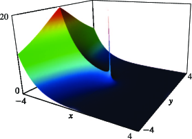
25: 6.3 Graphics

… ►

See accompanying text — Figure 6.3.1: The exponential integrals $E_{1}\left(x\right)$ and $\operatorname{Ei}\left(x\right)$ , $0<x\leq 2$ . Magnify

►

►For a graph of

\operatorname{li}\left(x\right)

see Figure 6.16.2. … ►

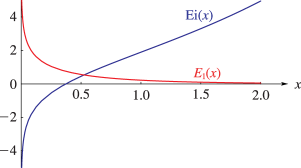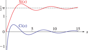26: 19.13 Integrals of Elliptic Integrals

§19.13 Integrals of Elliptic Integrals

… ►For definite and indefinite integrals of complete elliptic integrals see Byrd and Friedman (1971, pp. 610–612, 615), Prudnikov et al. (1990, §§1.11, 2.16), Glasser (1976), Bushell (1987), and Cvijović and Klinowski (1999). ►For definite and indefinite integrals of incomplete elliptic integrals see Byrd and Friedman (1971, pp. 613, 616), Prudnikov et al. (1990, §§1.10.2, 2.15.2), and Cvijović and Klinowski (1994). … ►

§19.13(iii) Laplace Transforms

►For direct and inverse Laplace transforms for the complete elliptic integrals

K\left(k\right)

E\left(k\right)

, and

D\left(k\right)

see Prudnikov et al. (1992a, §3.31) and Prudnikov et al. (1992b, §§3.29 and 4.3.33), respectively.

27: 6.20 Approximations

… ►

•

Hastings (1955) gives several minimax polynomial and rational approximations for $E_{1}\left(x\right)+\ln x$ , $xe^{x}E_{1}\left(x\right)$ , and the auxiliary functions $\mathrm{f}\left(x\right)$ and $\mathrm{g}\left(x\right)$ . These are included in Abramowitz and Stegun (1964, Ch. 5).

►

•

Cody and Thacher (1968) provides minimax rational approximations for $E_{1}\left(x\right)$ , with accuracies up to 20S.

►

•

Cody and Thacher (1969) provides minimax rational approximations for $\operatorname{Ei}\left(x\right)$ , with accuracies up to 20S.

►

•

MacLeod (1996b) provides rational approximations for the sine and cosine integrals and for the auxiliary functions $\mathrm{f}$ and $\mathrm{g}$ , with accuracies up to 20S.

… ►

•

Luke and Wimp (1963) covers $\operatorname{Ei}\left(x\right)$ for $x\leq-4$ (20D), and $\operatorname{Si}\left(x\right)$ and $\operatorname{Ci}\left(x\right)$ for $x\geq 4$ (20D).

…

28: 19.21 Connection Formulas

§19.21 Connection Formulas

►

§19.21(i) Complete Integrals

… ►The complete case of

R_{J}

can be expressed in terms of

R_{F}

and

R_{D}

: … ►

§19.21(ii) Incomplete Integrals

… ►

§19.21(iii) Change of Parameter of $R_{J}$

…

29: 6.19 Tables

… ►

§6.19(ii) Real Variables

►

•

Abramowitz and Stegun (1964, Chapter 5) includes $x^{-1}\operatorname{Si}\left(x\right)$ , $-x^{-2}\operatorname{Cin}\left(x\right)$ , $x^{-1}\operatorname{Ein}\left(x\right)$ , $-x^{-1}\operatorname{Ein}\left(-x\right)$ , $x=0(.01)0.5$ ; $\operatorname{Si}\left(x\right)$ , $\operatorname{Ci}\left(x\right)$ , $\operatorname{Ei}\left(x\right)$ , $E_{1}\left(x\right)$ , $x=0.5(.01)2$ ; $\operatorname{Si}\left(x\right)$ , $\operatorname{Ci}\left(x\right)$ , $xe^{-x}\operatorname{Ei}\left(x\right)$ , $xe^{x}E_{1}\left(x\right)$ , $x=2(.1)10$ ; $x\mathrm{f}\left(x\right)$ , $x^{2}\mathrm{g}\left(x\right)$ , $xe^{-x}\operatorname{Ei}\left(x\right)$ , $xe^{x}E_{1}\left(x\right)$ , $x^{-1}=0(.005)0.1$ ; $\operatorname{Si}\left(\pi x\right)$ , $\operatorname{Cin}\left(\pi x\right)$ , $x=0(.1)10$ . Accuracy varies but is within the range 8S–11S.

►

•

Zhang and Jin (1996, pp. 652, 689) includes $\operatorname{Si}\left(x\right)$ , $\operatorname{Ci}\left(x\right)$ , $x=0(.5)20(2)30$ , 8D; $\operatorname{Ei}\left(x\right)$ , $E_{1}\left(x\right)$ , $x=[0,100]$ , 8S.

… ►

•

Abramowitz and Stegun (1964, Chapter 5) includes the real and imaginary parts of $ze^{z}E_{1}\left(z\right)$ , $x=-19(1)20$ , $y=0(1)20$ , 6D; $e^{z}E_{1}\left(z\right)$ , $x=-4(.5)-2$ , $y=0(.2)1$ , 6D; $E_{1}\left(z\right)+\ln z$ , $x=-2(.5)2.5$ , $y=0(.2)1$ , 6D.

►

•

Zhang and Jin (1996, pp. 690–692) includes the real and imaginary parts of $E_{1}\left(z\right)$ , $\pm x=0.5,1,3,5,10,15,20,50,100$ , $y=0(.5)1(1)5(5)30,50,100$ , 8S.

30: 7.22 Methods of Computation

… ►

§7.22(i) Main Functions

►The methods available for computing the main functions in this chapter are analogous to those described in §§6.18(i)–6.18(iv) for the exponential integral and sine and cosine integrals, and similar comments apply. … ►

§7.22(ii) Goodwin–Staton Integral

… ►

§7.22(iii) Repeated Integrals of the Complementary Error Function

►The recursion scheme given by (7.18.1) and (7.18.7) can be used for computing

\mathop{\mathrm{i}^{n}\mathrm{erfc}}\left(x\right)

. …