SL(2,Z) bilinear transformation
(0.001 seconds)
41—50 of 814 matching pages
41: 13.23 Integrals
…
►
§13.23(i) Laplace and Mellin Transforms
… ►§13.23(ii) Fourier Transforms
… ►§13.23(iii) Hankel Transforms
… ► ►§13.23(iv) Integral Transforms in terms of Whittaker Functions
…42: 7.14 Integrals
…
►
Fourier Transform
… ►Laplace Transforms
… ►Laplace Transforms
… ►
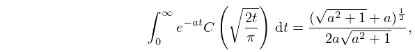
7.14.7
,
…
►For collections of integrals see Apelblat (1983, pp. 131–146), Erdélyi et al. (1954a, vol. 1, pp. 40, 96, 176–177), Geller and Ng (1971), Gradshteyn and Ryzhik (2000, §§5.4 and 6.28–6.32), Marichev (1983, pp. 184–189), Ng and Geller (1969), Oberhettinger (1974, pp. 138–139, 142–143), Oberhettinger (1990, pp. 48–52, 155–158), Oberhettinger and Badii (1973, pp. 171–172, 179–181), Prudnikov et al. (1986b, vol. 2, pp. 30–36, 93–143), Prudnikov et al. (1992a, §§3.7–3.8), and Prudnikov et al. (1992b, §§3.7–3.8).
…
43: 6.14 Integrals
…
►
§6.14(i) Laplace Transforms
… ►
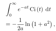
6.14.2
,
…
►
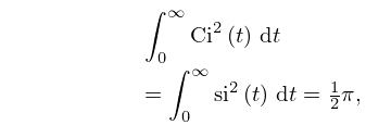
6.14.4
…
►
6.14.6
…
►For collections of integrals, see Apelblat (1983, pp. 110–123), Bierens de Haan (1939, pp. 373–374, 409, 479, 571–572, 637, 664–673, 680–682, 685–697), Erdélyi et al. (1954a, vol. 1, pp. 40–42, 96–98, 177–178, 325), Geller and Ng (1969), Gradshteyn and Ryzhik (2000, §§5.2–5.3 and 6.2–6.27), Marichev (1983, pp. 182–184), Nielsen (1906b), Oberhettinger (1974, pp. 139–141), Oberhettinger (1990, pp. 53–55 and 158–160), Oberhettinger and Badii (1973, pp. 172–179), Prudnikov et al. (1986b, vol. 2, pp. 24–29 and 64–92), Prudnikov et al. (1992a, §§3.4–3.6), Prudnikov et al. (1992b, §§3.4–3.6), and Watrasiewicz (1967).
44: 21.6 Products
…
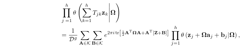
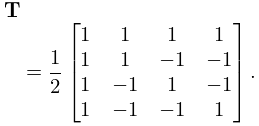
►Also, let be an arbitrary matrix.
…
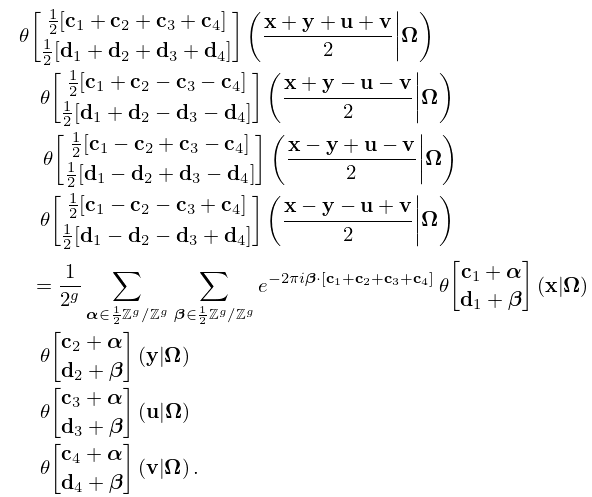
►
21.6.3
►where , , denote respectively the th columns of , , .
…
►
21.6.5
…
►
21.6.7
…
45: 18.8 Differential Equations
46: 29.21 Tables
…
►
•
►
•
Ince (1940a) tabulates the eigenvalues , (with and interchanged) for , , and . Precision is 4D.
Arscott and Khabaza (1962) tabulates the coefficients of the polynomials in Table 29.12.1 (normalized so that the numerically largest coefficient is unity, i.e. monic polynomials), and the corresponding eigenvalues for , . Equations from §29.6 can be used to transform to the normalization adopted in this chapter. Precision is 6S.
47: 1.16 Distributions
…
►
§1.16(vii) Fourier Transforms of Tempered Distributions
… ►Then its Fourier transform is … ►The Fourier transform of a tempered distribution is again a tempered distribution, and … ►§1.16(viii) Fourier Transforms of Special Distributions
… ►Since , we have …48: 13.10 Integrals
…
►
§13.10(ii) Laplace Transforms
… ►§13.10(iii) Mellin Transforms
… ►§13.10(iv) Fourier Transforms
… ►§13.10(v) Hankel Transforms
… ► …49: 2.6 Distributional Methods
…
►
