Riemann theta functions with characteristics

(0.007 seconds)

8 matching pages

1: 21.2 Definitions

… ►

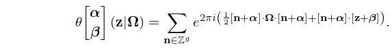
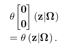
§21.2(ii) Riemann Theta Functions with Characteristics

… ►

21.2.5

\theta\genfrac{[}{]}{0.0pt}{}{\boldsymbol{{\alpha}}}{\boldsymbol{{\beta}}}% \left(\mathbf{z}\middle|\boldsymbol{{\Omega}}\right)=\sum_{\mathbf{n}\in{% \mathbb{Z}}^{g}}e^{2\pi i\left(\frac{1}{2}[\mathbf{n}+\boldsymbol{{\alpha}}]% \cdot\boldsymbol{{\Omega}}\cdot[\mathbf{n}+\boldsymbol{{\alpha}}]+[\mathbf{n}+% \boldsymbol{{\alpha}}]\cdot[\mathbf{z}+\boldsymbol{{\beta}}]\right)}.

ⓘ

Defines:: $\theta\genfrac{[}{]}{0.0pt}{}{\NVar{\boldsymbol{{\alpha}}}}{\NVar{\boldsymbol{% {\beta}}}}\left(\NVar{\mathbf{z}}\middle|\NVar{\boldsymbol{{\Omega}}}\right)$ : Riemann theta function with characteristics
Symbols:: $\pi$ : the ratio of the circumference of a circle to its diameter, $\in$ : element of, $\mathrm{e}$ : base of natural logarithm, $\mathrm{i}$ : imaginary unit, $\mathbb{Z}$ : set of all integers, $g$ : positive integer, $\boldsymbol{{\Omega}}$ : a Riemann matrix, $\boldsymbol{{\alpha}}$ : $g$ -dimensional vector and $\boldsymbol{{\beta}}$ : $g$ -dimensional vector
Permalink:: http://dlmf.nist.gov/21.2.E5
Encodings:: pMML, png, TeX
See also:: Annotations for §21.2(ii), §21.2 and Ch.21

►This function is referred to as a Riemann theta function with characteristics

\begin{bmatrix}\boldsymbol{{\alpha}}\\ \boldsymbol{{\beta}}\end{bmatrix}

. … ►

21.2.7

\theta\genfrac{[}{]}{0.0pt}{}{\boldsymbol{{0}}}{\boldsymbol{{0}}}\left(\mathbf% {z}\middle|\boldsymbol{{\Omega}}\right)=\theta\left(\mathbf{z}\middle|% \boldsymbol{{\Omega}}\right).

ⓘ

Symbols:: $\theta\left(\NVar{\mathbf{z}}\middle|\NVar{\boldsymbol{{\Omega}}}\right)$ : Riemann theta function, $\theta\genfrac{[}{]}{0.0pt}{}{\NVar{\boldsymbol{{\alpha}}}}{\NVar{\boldsymbol{% {\beta}}}}\left(\NVar{\mathbf{z}}\middle|\NVar{\boldsymbol{{\Omega}}}\right)$ : Riemann theta function with characteristics and $\boldsymbol{{\Omega}}$ : a Riemann matrix
Permalink:: http://dlmf.nist.gov/21.2.E7
Encodings:: pMML, png, TeX
See also:: Annotations for §21.2(ii), §21.2 and Ch.21

… ►For given

\boldsymbol{{\Omega}}

, there are

2^{2g}

g

-dimensional Riemann theta functions with half-period characteristics. …

2: 21.8 Abelian Functions

§21.8 Abelian Functions

… ►For every Abelian function, there is a positive integer

n

, such that the Abelian function can be expressed as a ratio of linear combinations of products with

n

factors of Riemann theta functions with characteristics that share a common period lattice. …

3: 21.3 Symmetry and Quasi-Periodicity

… ►

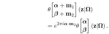
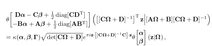
§21.3(ii) Riemann Theta Functions with Characteristics

… ►

21.3.4

\theta\genfrac{[}{]}{0.0pt}{}{\boldsymbol{{\alpha}}+\mathbf{m}_{1}}{% \boldsymbol{{\beta}}+\mathbf{m}_{2}}\left(\mathbf{z}\middle|\boldsymbol{{% \Omega}}\right)=e^{2\pi i\boldsymbol{{\alpha}}\cdot\mathbf{m}_{2}}\theta% \genfrac{[}{]}{0.0pt}{}{\boldsymbol{{\alpha}}}{\boldsymbol{{\beta}}}\left(% \mathbf{z}\middle|\boldsymbol{{\Omega}}\right).

ⓘ

Symbols:: $\theta\genfrac{[}{]}{0.0pt}{}{\NVar{\boldsymbol{{\alpha}}}}{\NVar{\boldsymbol{% {\beta}}}}\left(\NVar{\mathbf{z}}\middle|\NVar{\boldsymbol{{\Omega}}}\right)$ : Riemann theta function with characteristics, $\pi$ : the ratio of the circumference of a circle to its diameter, $\mathrm{e}$ : base of natural logarithm, $\mathrm{i}$ : imaginary unit, $\boldsymbol{{\Omega}}$ : a Riemann matrix, $\boldsymbol{{\alpha}}$ : $g$ -dimensional vector and $\boldsymbol{{\beta}}$ : $g$ -dimensional vector
Referenced by:: Erratum (V1.0.5) for Equation (21.3.4)
Permalink:: http://dlmf.nist.gov/21.3.E4
Encodings:: pMML, png, TeX
Errata (effective with 1.0.5):: Originally the vector $\mathbf{m}_{2}$ on the right-hand-side was given incorrectly as $\mathbf{m}_{1}$ .
Reported 2012-08-27 by Klaas Vantournhout
See also:: Annotations for §21.3(ii), §21.3 and Ch.21

… ► …For Riemann theta functions with half-period characteristics, ►

21.3.6

\theta\genfrac{[}{]}{0.0pt}{}{\boldsymbol{{\alpha}}}{\boldsymbol{{\beta}}}% \left(-\mathbf{z}\middle|\boldsymbol{{\Omega}}\right)=(-1)^{4\boldsymbol{{% \alpha}}\cdot\boldsymbol{{\beta}}}\theta\genfrac{[}{]}{0.0pt}{}{\boldsymbol{{% \alpha}}}{\boldsymbol{{\beta}}}\left(\mathbf{z}\middle|\boldsymbol{{\Omega}}% \right).

ⓘ

Symbols:: $\theta\genfrac{[}{]}{0.0pt}{}{\NVar{\boldsymbol{{\alpha}}}}{\NVar{\boldsymbol{% {\beta}}}}\left(\NVar{\mathbf{z}}\middle|\NVar{\boldsymbol{{\Omega}}}\right)$ : Riemann theta function with characteristics, $\boldsymbol{{\Omega}}$ : a Riemann matrix, $\boldsymbol{{\alpha}}$ : $g$ -dimensional vector and $\boldsymbol{{\beta}}$ : $g$ -dimensional vector
Permalink:: http://dlmf.nist.gov/21.3.E6
Encodings:: pMML, png, TeX
See also:: Annotations for §21.3(ii), §21.3 and Ch.21

…

4: 21.1 Special Notation

… ►Uppercase boldface letters are

g\times g

real or complex matrices. ►The main functions treated in this chapter are the Riemann theta functions

\theta\left(\mathbf{z}\middle|\boldsymbol{{\Omega}}\right)

, and the Riemann theta functions with characteristics

\theta\genfrac{[}{]}{0.0pt}{}{\boldsymbol{{\alpha}}}{\boldsymbol{{\beta}}}% \left(\mathbf{z}\middle|\boldsymbol{{\Omega}}\right)

. ►The function

\Theta(\boldsymbol{{\phi}}|\mathbf{B})=\theta\left(\boldsymbol{{\phi}}/(2\pi i% )\middle|\mathbf{B}/(2\pi i)\right)

is also commonly used; see, for example, Belokolos et al. (1994, §2.5), Dubrovin (1981), and Fay (1973, Chapter 1).

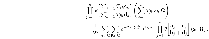
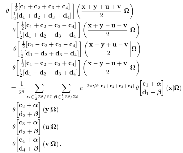
5: 21.6 Products

… ►On using theta functions with characteristics, it becomes ►

21.6.4

\prod_{j=1}^{h}\theta\genfrac{[}{]}{0.0pt}{}{\sum_{k=1}^{h}T_{jk}\mathbf{c}_{k% }}{\sum_{k=1}^{h}T_{jk}\mathbf{d}_{k}}\left(\sum_{k=1}^{h}T_{jk}\mathbf{z}_{k}% \middle|\boldsymbol{{\Omega}}\right)=\frac{1}{\mathcal{D}^{g}}\sum_{\mathbf{A}% \in\mathcal{K}}\sum_{\mathbf{B}\in\mathcal{K}}e^{-2\pi i\sum_{j=1}^{h}\mathbf{% b}_{j}\cdot\mathbf{c}_{j}}\prod_{j=1}^{h}\theta\genfrac{[}{]}{0.0pt}{}{\mathbf% {a}_{j}+\mathbf{c}_{j}}{\mathbf{b}_{j}+\mathbf{d}_{j}}\left(\mathbf{z}_{j}% \middle|\boldsymbol{{\Omega}}\right),

ⓘ

Symbols:: $\theta\genfrac{[}{]}{0.0pt}{}{\NVar{\boldsymbol{{\alpha}}}}{\NVar{\boldsymbol{% {\beta}}}}\left(\NVar{\mathbf{z}}\middle|\NVar{\boldsymbol{{\Omega}}}\right)$ : Riemann theta function with characteristics, $\pi$ : the ratio of the circumference of a circle to its diameter, $\in$ : element of, $\mathrm{e}$ : base of natural logarithm, $\mathrm{i}$ : imaginary unit, $g$ : positive integer, $h$ : positive integer, $\boldsymbol{{\Omega}}$ : a Riemann matrix, $T_{jk}$ : element, $\mathcal{K}$ : set of matrices and $\mathcal{D}$ : number of elements
Permalink:: http://dlmf.nist.gov/21.6.E4
Encodings:: pMML, png, TeX
See also:: Annotations for §21.6(i), §21.6 and Ch.21

… ►

21.6.7

\theta\genfrac{[}{]}{0.0pt}{}{\tfrac{1}{2}[\mathbf{c}_{1}+\mathbf{c}_{2}+% \mathbf{c}_{3}+\mathbf{c}_{4}]}{\tfrac{1}{2}[\mathbf{d}_{1}+\mathbf{d}_{2}+% \mathbf{d}_{3}+\mathbf{d}_{4}]}\left(\frac{\mathbf{x}+\mathbf{y}+\mathbf{u}+% \mathbf{v}}{2}\middle|\boldsymbol{{\Omega}}\right)\theta\genfrac{[}{]}{0.0pt}{% }{\tfrac{1}{2}[\mathbf{c}_{1}+\mathbf{c}_{2}-\mathbf{c}_{3}-\mathbf{c}_{4}]}{% \tfrac{1}{2}[\mathbf{d}_{1}+\mathbf{d}_{2}-\mathbf{d}_{3}-\mathbf{d}_{4}]}% \left(\frac{\mathbf{x}+\mathbf{y}-\mathbf{u}-\mathbf{v}}{2}\middle|\boldsymbol% {{\Omega}}\right)\*\theta\genfrac{[}{]}{0.0pt}{}{\tfrac{1}{2}[\mathbf{c}_{1}-% \mathbf{c}_{2}+\mathbf{c}_{3}-\mathbf{c}_{4}]}{\tfrac{1}{2}[\mathbf{d}_{1}-% \mathbf{d}_{2}+\mathbf{d}_{3}-\mathbf{d}_{4}]}\left(\frac{\mathbf{x}-\mathbf{y% }+\mathbf{u}-\mathbf{v}}{2}\middle|\boldsymbol{{\Omega}}\right)\theta\genfrac{% [}{]}{0.0pt}{}{\tfrac{1}{2}[\mathbf{c}_{1}-\mathbf{c}_{2}-\mathbf{c}_{3}+% \mathbf{c}_{4}]}{\tfrac{1}{2}[\mathbf{d}_{1}-\mathbf{d}_{2}-\mathbf{d}_{3}+% \mathbf{d}_{4}]}\left(\frac{\mathbf{x}-\mathbf{y}-\mathbf{u}+\mathbf{v}}{2}% \middle|\boldsymbol{{\Omega}}\right)\\ =\frac{1}{2^{g}}\sum_{\boldsymbol{{\alpha}}\in\frac{1}{2}{\mathbb{Z}}^{g}/{% \mathbb{Z}}^{g}}\,\sum_{\boldsymbol{{\beta}}\in\frac{1}{2}{\mathbb{Z}}^{g}/{% \mathbb{Z}}^{g}}e^{-2\pi i\boldsymbol{{\beta}}\cdot[\mathbf{c}_{1}+\mathbf{c}_% {2}+\mathbf{c}_{3}+\mathbf{c}_{4}]}\*\theta\genfrac{[}{]}{0.0pt}{}{\mathbf{c}_% {1}+\boldsymbol{{\alpha}}}{\mathbf{d}_{1}+\boldsymbol{{\beta}}}\left(\mathbf{x% }\middle|\boldsymbol{{\Omega}}\right)\theta\genfrac{[}{]}{0.0pt}{}{\mathbf{c}_% {2}+\boldsymbol{{\alpha}}}{\mathbf{d}_{2}+\boldsymbol{{\beta}}}\left(\mathbf{y% }\middle|\boldsymbol{{\Omega}}\right)\theta\genfrac{[}{]}{0.0pt}{}{\mathbf{c}_% {3}+\boldsymbol{{\alpha}}}{\mathbf{d}_{3}+\boldsymbol{{\beta}}}\left(\mathbf{u% }\middle|\boldsymbol{{\Omega}}\right)\theta\genfrac{[}{]}{0.0pt}{}{\mathbf{c}_% {4}+\boldsymbol{{\alpha}}}{\mathbf{d}_{4}+\boldsymbol{{\beta}}}\left(\mathbf{v% }\middle|\boldsymbol{{\Omega}}\right).

ⓘ

Symbols:: $\theta\genfrac{[}{]}{0.0pt}{}{\NVar{\boldsymbol{{\alpha}}}}{\NVar{\boldsymbol{% {\beta}}}}\left(\NVar{\mathbf{z}}\middle|\NVar{\boldsymbol{{\Omega}}}\right)$ : Riemann theta function with characteristics, $\pi$ : the ratio of the circumference of a circle to its diameter, $\in$ : element of, $\mathrm{e}$ : base of natural logarithm, $\mathrm{i}$ : imaginary unit, $\mathbb{Z}$ : set of all integers, $g$ : positive integer, $\boldsymbol{{\Omega}}$ : a Riemann matrix, $\boldsymbol{{\alpha}}$ : $g$ -dimensional vector and $\boldsymbol{{\beta}}$ : $g$ -dimensional vector
Permalink:: http://dlmf.nist.gov/21.6.E7
Encodings:: pMML, png, TeX
See also:: Annotations for §21.6(i), §21.6(i), §21.6 and Ch.21

►

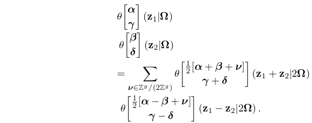
§21.6(ii) Addition Formulas

… ►

21.6.8

\theta\genfrac{[}{]}{0.0pt}{}{\boldsymbol{{\alpha}}}{\boldsymbol{{\gamma}}}% \left(\mathbf{z}_{1}\middle|\boldsymbol{{\Omega}}\right)\theta\genfrac{[}{]}{0% .0pt}{}{\boldsymbol{{\beta}}}{\boldsymbol{{\delta}}}\left(\mathbf{z}_{2}% \middle|\boldsymbol{{\Omega}}\right)=\sum_{\boldsymbol{{\nu}}\in{\mathbb{Z}}^{% g}/\left(2{\mathbb{Z}}^{g}\right)}\theta\genfrac{[}{]}{0.0pt}{}{\frac{1}{2}[% \boldsymbol{{\alpha}}+\boldsymbol{{\beta}}+\boldsymbol{{\nu}}]}{\boldsymbol{{% \gamma}}+\boldsymbol{{\delta}}}\left(\mathbf{z}_{1}+\mathbf{z}_{2}\middle|2% \boldsymbol{{\Omega}}\right)\*\theta\genfrac{[}{]}{0.0pt}{}{\frac{1}{2}[% \boldsymbol{{\alpha}}-\boldsymbol{{\beta}}+\boldsymbol{{\nu}}]}{\boldsymbol{{% \gamma}}-\boldsymbol{{\delta}}}\left(\mathbf{z}_{1}-\mathbf{z}_{2}\middle|2% \boldsymbol{{\Omega}}\right).

ⓘ

Symbols:: $\theta\genfrac{[}{]}{0.0pt}{}{\NVar{\boldsymbol{{\alpha}}}}{\NVar{\boldsymbol{% {\beta}}}}\left(\NVar{\mathbf{z}}\middle|\NVar{\boldsymbol{{\Omega}}}\right)$ : Riemann theta function with characteristics, $\in$ : element of, $\mathbb{Z}$ : set of all integers, $g$ : positive integer, $\boldsymbol{{\Omega}}$ : a Riemann matrix, $\boldsymbol{{\alpha}}$ : $g$ -dimensional vector, $\boldsymbol{{\beta}}$ : $g$ -dimensional vector, $\boldsymbol{{\delta}}$ : $g$ -dimensional vector and $\boldsymbol{{\gamma}}$ : $g$ -dimensional vector
Permalink:: http://dlmf.nist.gov/21.6.E8
Encodings:: pMML, png, TeX
See also:: Annotations for §21.6(ii), §21.6 and Ch.21

…

6: 21.5 Modular Transformations

… ►

§21.5(ii) Riemann Theta Functions with Characteristics

►

21.5.9

\theta\genfrac{[}{]}{0.0pt}{}{\mathbf{D}\boldsymbol{{\alpha}}-\mathbf{C}% \boldsymbol{{\beta}}+\tfrac{1}{2}\operatorname{diag}[\mathbf{C}\mathbf{D}^{% \mathrm{T}}]}{-\mathbf{B}\boldsymbol{{\alpha}}+\mathbf{A}\boldsymbol{{\beta}}+% \tfrac{1}{2}\operatorname{diag}[\mathbf{A}\mathbf{B}^{\mathrm{T}}]}\left(\left% [[\mathbf{C}\boldsymbol{{\Omega}}+\mathbf{D}]^{-1}\right]^{\mathrm{T}}\mathbf{% z}\middle|[\mathbf{A}\boldsymbol{{\Omega}}+\mathbf{B}][\mathbf{C}\boldsymbol{{% \Omega}}+\mathbf{D}]^{-1}\right)=\kappa(\boldsymbol{{\alpha}},\boldsymbol{{% \beta}},\boldsymbol{{\Gamma}})\sqrt{\det[\mathbf{C}\boldsymbol{{\Omega}}+% \mathbf{D}]}e^{\pi i\mathbf{z}\cdot\left[[\mathbf{C}\boldsymbol{{\Omega}}+% \mathbf{D}]^{-1}\mathbf{C}\right]\cdot\mathbf{z}}\theta\genfrac{[}{]}{0.0pt}{}% {\boldsymbol{{\alpha}}}{\boldsymbol{{\beta}}}\left(\mathbf{z}\middle|% \boldsymbol{{\Omega}}\right),

ⓘ

Symbols:: $\theta\genfrac{[}{]}{0.0pt}{}{\NVar{\boldsymbol{{\alpha}}}}{\NVar{\boldsymbol{% {\beta}}}}\left(\NVar{\mathbf{z}}\middle|\NVar{\boldsymbol{{\Omega}}}\right)$ : Riemann theta function with characteristics, $\pi$ : the ratio of the circumference of a circle to its diameter, $\det$ : determinant, $\mathrm{e}$ : base of natural logarithm, $\mathrm{i}$ : imaginary unit, $\NVar{\mathbf{A}}^{\mathrm{T}}$ : transpose of matrix, $\boldsymbol{{\Omega}}$ : a Riemann matrix, $\boldsymbol{{\alpha}}$ : $g$ -dimensional vector, $\boldsymbol{{\beta}}$ : $g$ -dimensional vector, $\operatorname{diag}\mathbf{A}$ : Transpose of $[A_{11},A_{22},\ldots,A_{gg}]$ and Matrix $\boldsymbol{{\Gamma}}$
Permalink:: http://dlmf.nist.gov/21.5.E9
Encodings:: pMML, png, TeX
See also:: Annotations for §21.5(ii), §21.5 and Ch.21

…

7: 21.7 Riemann Surfaces

… ►

§21.7(ii) Fay’s Trisecant Identity

… ►

21.7.8

\zeta=\sum_{j=1}^{g}\omega_{j}\frac{\partial}{\partial z_{j}}\theta\genfrac{[}% {]}{0.0pt}{}{\boldsymbol{{\alpha}}}{\boldsymbol{{\beta}}}\left(\mathbf{z}% \middle|\boldsymbol{{\Omega}}\right)\Big{|}_{\mathbf{z}=\boldsymbol{{0}}}.

ⓘ

Symbols:: $\theta\genfrac{[}{]}{0.0pt}{}{\NVar{\boldsymbol{{\alpha}}}}{\NVar{\boldsymbol{% {\beta}}}}\left(\NVar{\mathbf{z}}\middle|\NVar{\boldsymbol{{\Omega}}}\right)$ : Riemann theta function with characteristics, $\frac{\partial\NVar{f}}{\partial\NVar{x}}$ : partial derivative of $f$ with respect to $x$ , $\,\partial\NVar{x}$ : partial differential of $x$ , $g$ : positive integer, $\boldsymbol{{\Omega}}$ : a Riemann matrix, $\boldsymbol{{\alpha}}$ : $g$ -dimensional vector, $\boldsymbol{{\beta}}$ : $g$ -dimensional vector and $\omega$ : differential
Permalink:: http://dlmf.nist.gov/21.7.E8
Encodings:: pMML, png, TeX
See also:: Annotations for §21.7(ii), §21.7 and Ch.21

… ►

21.7.9

E(P_{1},P_{2})=\theta\genfrac{[}{]}{0.0pt}{}{\boldsymbol{{\alpha}}}{% \boldsymbol{{\beta}}}\left(\int_{P_{1}}^{P_{2}}\boldsymbol{{\omega}}\middle|% \boldsymbol{{\Omega}}\right)\Bigg{/}\left(\sqrt{\zeta(P_{1})}\sqrt{\zeta(P_{2}% )}\right),

ⓘ

Defines:: $E(\NVar{P_{1}},\NVar{P_{2}})$ : prime form (locally)
Symbols:: $\theta\genfrac{[}{]}{0.0pt}{}{\NVar{\boldsymbol{{\alpha}}}}{\NVar{\boldsymbol{% {\beta}}}}\left(\NVar{\mathbf{z}}\middle|\NVar{\boldsymbol{{\Omega}}}\right)$ : Riemann theta function with characteristics, $\int$ : integral, $\boldsymbol{{\Omega}}$ : a Riemann matrix, $\boldsymbol{{\alpha}}$ : $g$ -dimensional vector, $\boldsymbol{{\beta}}$ : $g$ -dimensional vector, $P_{1},P_{2}$ : points and $\boldsymbol{{\omega}}$ : vector of differentials
Permalink:: http://dlmf.nist.gov/21.7.E9
Encodings:: pMML, png, TeX
See also:: Annotations for §21.7(ii), §21.7 and Ch.21

… ► ►

§21.7(iii) Frobenius’ Identity

…

8: Bibliography

… ►

C. Adiga, B. C. Berndt, S. Bhargava, and G. N. Watson (1985) Chapter

16

of Ramanujan’s second notebook: Theta-functions and

q

-series. Mem. Amer. Math. Soc. 53 (315), pp. v+85.

ⓘ

External Links:: ISSN 0065-9266, MathReview (R. A. Askey), ZentralBlatt
Referenced by:: §20.11(ii).
Encodings:: BibTeX

… ►

G. Allasia and R. Besenghi (1989) Numerical Calculation of the Riemann Zeta Function and Generalizations by Means of the Trapezoidal Rule. In Numerical and Applied Mathematics, Part II (Paris, 1988), C. Brezinski (Ed.), IMACS Ann. Comput. Appl. Math., Vol. 1, pp. 467–472.

ⓘ

External Links:: MathReview
Referenced by:: §25.18(i).
Encodings:: BibTeX

… ►

G. E. Andrews (1966a) On basic hypergeometric series, mock theta functions, and partitions. II. Quart. J. Math. Oxford Ser. (2) 17, pp. 132–143.

ⓘ

External Links:: Document, MathReview (B. R. Bhonsle), ZentralBlatt
Referenced by:: §17.6(ii).
Encodings:: BibTeX

… ►

T. M. Apostol and T. H. Vu (1984) Dirichlet series related to the Riemann zeta function. J. Number Theory 19 (1), pp. 85–102.

ⓘ

External Links:: ISSN 0022-314X, Document, MathReview (Kai Man Tsang), ZentralBlatt
Referenced by:: (25.16.10), (25.16.11), (25.16.12), (25.16.14), (25.16.15), (25.16.5), (25.16.6), (25.16.7), (25.16.8), (25.16.9), §25.16(ii), §25.16(ii), §25.16.
Encodings:: BibTeX

… ►

T. M. Apostol (1985a) Formulas for higher derivatives of the Riemann zeta function. Math. Comp. 44 (169), pp. 223–232.

ⓘ

External Links:: ISSN 0025-5718, FullText, MathReview (Aleksandar Ivić), ZentralBlatt
Referenced by:: (25.11.19), (25.11.20), (25.11.6), §25.11(vi), §25.18(i), (25.4.5), (25.4.6), §25.4, (25.6.11), (25.6.12), (25.6.13), (25.6.14), §25.6(ii), §25.6.
Encodings:: BibTeX

…