Pochhammer%20double-loop%20contour

SearchAdvancedHelp

(0.003 seconds)

11—20 of 260 matching pages

11: 17.13 Integrals

… ►

17.13.1 $${\int }_{-c}^d\frac{{(-qx/c;q)}_{\mathrm{\infty }}{(qx/d;q)}_{\mathrm{\infty }}}{{(-ax/c;q)}_{\mathrm{\infty }}{(bx/d;q)}_{\mathrm{\infty }}}{d}_{q}x=\frac{(1-q){(q;q)}_{\mathrm{\infty }}{(ab;q)}_{\mathrm{\infty }}cd{(-c/d;q)}_{\mathrm{\infty }}{(-d/c;q)}_{\mathrm{\infty }}}{{(a;q)}_{\mathrm{\infty }}{(b;q)}_{\mathrm{\infty }}(c+d){(-bc/d;q)}_{\mathrm{\infty }}{(-ad/c;q)}_{\mathrm{\infty }}},$$

ⓘ

Symbols:

$\int$: integral, ${(a;q)}_n$: $q$-Pochhammer symbol (or $q$-shifted factorial), $d_{q}x$: $q$-differential, $q$: complex base and $x$: real variable

Permalink:

http://dlmf.nist.gov/17.13.E1

Encodings:

pMML, png, TeX

See also:

Annotations for §17.13 and Ch.17

… ►

17.13.2 $${\int }_{-c}^d\frac{{(-qx/c;q)}_{\mathrm{\infty }}{(qx/d;q)}_{\mathrm{\infty }}}{{(-x{q}^{\alpha }/c;q)}_{\mathrm{\infty }}{(x{q}^{\beta }/d;q)}_{\mathrm{\infty }}}{d}_{q}x=\frac{{\mathrm{\Gamma }}_q\left(\alpha \right){\mathrm{\Gamma }}_q\left(\beta \right)}{{\mathrm{\Gamma }}_q\left(\alpha +\beta \right)}\frac{cd}{c+d}\frac{{(-c/d;q)}_{\mathrm{\infty }}{(-d/c;q)}_{\mathrm{\infty }}}{{(-q^{\beta }c/d;q)}_{\mathrm{\infty }}{(-q^{\alpha }d/c;q)}_{\mathrm{\infty }}}.$$

ⓘ

Symbols:

$\int$: integral, ${\mathrm{\Gamma }}_q\left(z\right)$: $q$-gamma function, ${(a;q)}_n$: $q$-Pochhammer symbol (or $q$-shifted factorial), $d_{q}x$: $q$-differential, $q$: complex base and $x$: real variable

Permalink:

http://dlmf.nist.gov/17.13.E2

Encodings:

pMML, png, TeX

See also:

Annotations for §17.13 and Ch.17

… ►

17.13.3 $${\int }_0^{\mathrm{\infty }}{t}^{\alpha -1}\frac{{(-t{q}^{\alpha +\beta };q)}_{\mathrm{\infty }}}{{(-t;q)}_{\mathrm{\infty }}}dt=\frac{\mathrm{\Gamma }\left(\alpha \right)\mathrm{\Gamma }\left(1-\alpha \right){\mathrm{\Gamma }}_q\left(\beta \right)}{{\mathrm{\Gamma }}_q\left(1-\alpha \right){\mathrm{\Gamma }}_q\left(\alpha +\beta \right)},$$

ⓘ

Symbols:

$\mathrm{\Gamma }\left(z\right)$: gamma function, $dx$: differential of $x$ , $\int$: integral, ${\mathrm{\Gamma }}_q\left(z\right)$: $q$-gamma function, ${(a;q)}_n$: $q$-Pochhammer symbol (or $q$-shifted factorial) and $q$: complex base

Referenced by:

Erratum (V1.0.1) for Equation (17.13.3)

Permalink:

http://dlmf.nist.gov/17.13.E3

Encodings:

pMML, png, TeX

Errata (effective with 1.0.1):

Originally the differential was identified incorrectly as a $q$-differential; the correct differential is $dt$.

See also:

Annotations for §17.13, §17.13 and Ch.17

►

17.13.4 $${\int }_0^{\mathrm{\infty }}{t}^{\alpha -1}\frac{{(-ct{q}^{\alpha +\beta };q)}_{\mathrm{\infty }}}{{(-ct;q)}_{\mathrm{\infty }}}{d}_{q}t=\frac{{\mathrm{\Gamma }}_q\left(\alpha \right){\mathrm{\Gamma }}_q\left(\beta \right){(-c{q}^{\alpha };q)}_{\mathrm{\infty }}{(-q^{1-\alpha }/c;q)}_{\mathrm{\infty }}}{{\mathrm{\Gamma }}_q\left(\alpha +\beta \right){(-c;q)}_{\mathrm{\infty }}{(-q/c;q)}_{\mathrm{\infty }}}.$$

ⓘ

Symbols:

$\int$: integral, ${\mathrm{\Gamma }}_q\left(z\right)$: $q$-gamma function, ${(a;q)}_n$: $q$-Pochhammer symbol (or $q$-shifted factorial), $d_{q}x$: $q$-differential and $q$: complex base

Permalink:

http://dlmf.nist.gov/17.13.E4

Encodings:

pMML, png, TeX

See also:

Annotations for §17.13, §17.13 and Ch.17

…

12: 16.13 Appell Functions

… ►

16.13.1 $$F_1(\alpha ;\beta ,{\beta }^{\prime };\gamma ;x,y)=\sum _{m,n=0}^{\mathrm{\infty }}\frac{{\left(\alpha \right)}_{m+n}{\left(\beta \right)}_m{\left({\beta }^{\prime }\right)}_n}{{\left(\gamma \right)}_{m+n}m!n!}{x}^m{y}^n,$$ ,

ⓘ

Defines:

$F_1(\alpha ;\beta ,{\beta }^{\prime };\gamma ;x,y)$: first Appell function

Symbols:

${\left(a\right)}_n$: Pochhammer’s symbol (or shifted factorial) and $!$: factorial (as in $n!$)

Permalink:

http://dlmf.nist.gov/16.13.E1

Encodings:

pMML, png, TeX

See also:

Annotations for §16.13 and Ch.16

►

16.13.2 $$F_2(\alpha ;\beta ,{\beta }^{\prime };\gamma ,{\gamma }^{\prime };x,y)=\sum _{m,n=0}^{\mathrm{\infty }}\frac{{\left(\alpha \right)}_{m+n}{\left(\beta \right)}_m{\left({\beta }^{\prime }\right)}_n}{{\left(\gamma \right)}_m{\left({\gamma }^{\prime }\right)}_{n}m!n!}{x}^m{y}^n,$$ ,

ⓘ

Defines:

$F_2(\alpha ;\beta ,{\beta }^{\prime };\gamma ,{\gamma }^{\prime };x,y)$: second Appell function

Symbols:

${\left(a\right)}_n$: Pochhammer’s symbol (or shifted factorial) and $!$: factorial (as in $n!$)

Permalink:

http://dlmf.nist.gov/16.13.E2

Encodings:

pMML, png, TeX

See also:

Annotations for §16.13 and Ch.16

►

16.13.3 $$F_3(\alpha ,{\alpha }^{\prime };\beta ,{\beta }^{\prime };\gamma ;x,y)=\sum _{m,n=0}^{\mathrm{\infty }}\frac{{\left(\alpha \right)}_m{\left({\alpha }^{\prime }\right)}_n{\left(\beta \right)}_m{\left({\beta }^{\prime }\right)}_n}{{\left(\gamma \right)}_{m+n}m!n!}{x}^m{y}^n,$$ ,

ⓘ

Defines:

$F_3(\alpha ,{\alpha }^{\prime };\beta ,{\beta }^{\prime };\gamma ;x,y)$: third Appell function

Symbols:

${\left(a\right)}_n$: Pochhammer’s symbol (or shifted factorial) and $!$: factorial (as in $n!$)

Permalink:

http://dlmf.nist.gov/16.13.E3

Encodings:

pMML, png, TeX

See also:

Annotations for §16.13 and Ch.16

►

16.13.4 $$F_4(\alpha ,\beta ;\gamma ,{\gamma }^{\prime };x,y)=\sum _{m,n=0}^{\mathrm{\infty }}\frac{{\left(\alpha \right)}_{m+n}{\left(\beta \right)}_{m+n}}{{\left(\gamma \right)}_m{\left({\gamma }^{\prime }\right)}_{n}m!n!}{x}^m{y}^n,$$ .

ⓘ

Defines:

$F_4(\alpha ,\beta ;\gamma ,{\gamma }^{\prime };x,y)$: fourth Appell function

Symbols:

${\left(a\right)}_n$: Pochhammer’s symbol (or shifted factorial) and $!$: factorial (as in $n!$)

Permalink:

http://dlmf.nist.gov/16.13.E4

Encodings:

pMML, png, TeX

See also:

Annotations for §16.13 and Ch.16

…

13: 17.2 Calculus

… ►For $n=0,1,2,\mathrm{\dots }$, … … ►For properties of the function $f\left(q\right)=q^{-1/24}\eta \left(\frac{\ln q}{2\pi \mathrm{i}}\right)={(q;q)}_{\mathrm{\infty }}$ see §27.14. … ►

17.2.18 $${(a{q}^k;q)}_{n-k}=\frac{{(a;q)}_n}{{(a;q)}_k}.$$

ⓘ

Symbols:

${(a;q)}_n$: $q$-Pochhammer symbol (or $q$-shifted factorial), $k$: nonnegative integer, $q$: complex base and $n$: nonnegative integer

Permalink:

http://dlmf.nist.gov/17.2.E18

Encodings:

pMML, png, TeX

See also:

Annotations for §17.2(i), §17.2 and Ch.17

… ►

17.2.21 $${(a^2;q^2)}_n={(a;q)}_n{(-a;q)}_n,$$

ⓘ

Symbols:

${(a;q)}_n$: $q$-Pochhammer symbol (or $q$-shifted factorial), $q$: complex base and $n$: nonnegative integer

Permalink:

http://dlmf.nist.gov/17.2.E21

Encodings:

pMML, png, TeX

See also:

Annotations for §17.2(i), §17.2 and Ch.17

…

14: 25.5 Integral Representations

… ►

25.5.7 $$\zeta \left(s\right)=\frac{1}{2}+\frac{1}{s-1}+\sum _{m=1}^n\frac{B_{2m}}{(2m)!}{\left(s\right)}_{2m-1}+\frac{1}{\mathrm{\Gamma }\left(s\right)}{\int }_0^{\mathrm{\infty }}\left(\frac{1}{{\mathrm{e}}^x-1}-\frac{1}{x}+\frac{1}{2}-\sum _{m=1}^n\frac{B_{2m}}{(2m)!}{x}^{2m-1}\right)\frac{x^{s-1}}{{\mathrm{e}}^x}dx,$$ $\mathrm{\Re }s>-(2n+1)$, $n=1,2,3,\mathrm{\dots }$.

ⓘ

Symbols:

$B_n$: Bernoulli numbers, $O\left(x\right)$: order not exceeding, $\mathrm{\Gamma }\left(z\right)$: gamma function, ${\left(a\right)}_n$: Pochhammer’s symbol (or shifted factorial), $\zeta \left(s\right)$: Riemann zeta function, $dx$: differential of $x$ , $\mathrm{e}$: base of natural logarithm, $!$: factorial (as in $n!$), $\int$: integral, $\mathrm{\Re }$: real part, $m$: nonnegative integer, $n$: nonnegative integer, $x$: real variable and $s$: complex variable

Keywords:

improper integral, integral representation

Proof sketch:

Derivable from (25.5.6) by adding and subtracting ${\sum }_{m=1}^n{B}_{2m}{x}^{2m-1}/(2m)!$ in the integrand, using (5.2.1), (5.2.5), and recognizing that ${({\mathrm{e}}^x-1)}^{-1}-x^{-1}+1/2-{\sum }_{m=1}^n{B}_{2m}{x}^{2m-1}/(2m)!=O\left(x^{2n+1}\right)$ as $x\to 0$, demonstrating the region of convergence.

Referenced by:

Erratum (V1.0.9) for Chapters 7, 25

Permalink:

http://dlmf.nist.gov/25.5.E7

Encodings:

pMML, png, TeX

Notational Change (effective with 1.0.9):

We have rewritten the original summation ${\sum }_{m=1}^n\frac{B_{2m}}{(2m)!}\frac{\mathrm{\Gamma }\left(s+2m-1\right)}{\mathrm{\Gamma }\left(s\right)}$ more concisely as ${\sum }_{m=1}^n\frac{B_{2m}}{(2m)!}{\left(s\right)}_{2m-1}$ using the Pochhammer symbol.

See also:

Annotations for §25.5(i), §25.5 and Ch.25

… ►

§25.5(iii) Contour Integrals

►

25.5.20 $$\zeta \left(s\right)=\frac{\mathrm{\Gamma }\left(1-s\right)}{2\pi \mathrm{i}}{\int }_{-\mathrm{\infty }}^{(0+)}\frac{z^{s-1}}{{\mathrm{e}}^{-z}-1}dz,$$ $s\ne 1,2,\mathrm{\dots }$,

ⓘ

Symbols:

$\mathrm{\Gamma }\left(z\right)$: gamma function, $\zeta \left(s\right)$: Riemann zeta function, $\pi$: the ratio of the circumference of a circle to its diameter, $dx$: differential of $x$ , $\mathrm{e}$: base of natural logarithm, $\mathrm{i}$: imaginary unit, $\int$: integral, $a$: real or complex parameter, $s$: complex variable and $z$: complex variable

Keywords:

contour integral, integral representation

Sources:

Apostol (1976, (6), p. 253); with $a=1$; Erdélyi et al. (1953a, (1.12.9), p. 32); with $z=-t$

A&S Ref:

23.2.4 (in slightly different form)

Referenced by:

§25.11(vii)

Permalink:

http://dlmf.nist.gov/25.5.E20

Encodings:

pMML, png, TeX

See also:

Annotations for §25.5(iii), §25.5 and Ch.25

►where the integration contour is a loop around the negative real axis; it starts at $-\mathrm{\infty }$, encircles the origin once in the positive direction without enclosing any of the points $z=\pm 2\pi \mathrm{i}$, $\pm 4\pi \mathrm{i}$, …, and returns to $-\mathrm{\infty }$. …The contour here is any loop that encircles the origin in the positive direction not enclosing any of the points $\pm \pi \mathrm{i}$, $\pm 3\pi \mathrm{i}$, ….

15: 17.11 Transformations of $q$-Appell Functions

… ►

17.11.1 $${\mathrm{\Phi }}^{(1)}(a;b,b^{\prime };c;q;x,y)=\frac{{(a,bx,b^{\prime }y;q)}_{\mathrm{\infty }}}{{(c,x,y;q)}_{\mathrm{\infty }}}{}_3{}^{}\varphi _2^{}(\genfrac{}{}{0pt}{}{c/a,x,y}{bx,b^{\prime }y};q,a),$$

ⓘ

Symbols:

${\mathrm{\Phi }}^{(1)}(a;b,b^{\prime };c;q;x,y)$: first $q$-Appell function, ${}_{r+1}{}^{}\varphi _s^{}(a_0,\mathrm{\dots },a_r;b_1,\mathrm{\dots },b_s;q,z)$ or ${}_{r+1}{}^{}\varphi _s^{}(\genfrac{}{}{0pt}{}{a_0,\mathrm{\dots },a_r}{b_1,\mathrm{\dots },b_s};q,z)$: basic hypergeometric (or $q$-hypergeometric) function, ${(a_1,a_2,\mathrm{\dots },a_r;q)}_n$: multiple $q$-Pochhammer symbol, $q$: complex base, $x$: real variable and $y$: real variable

Referenced by:

§17.11, Erratum (V1.0.10) for Section 17.1

Permalink:

http://dlmf.nist.gov/17.11.E1

Encodings:

pMML, png, TeX

Correction (effective with 1.0.10):

The notation for ${\mathrm{\Phi }}^{(1)}$ has been updated to that of Gasper and Rahman (2004) to explicitly include the $q$ argument.

See also:

Annotations for §17.11 and Ch.17

►

17.11.2 $${\mathrm{\Phi }}^{(2)}(a;b,b^{\prime };c,c^{\prime };q;x,y)=\frac{{(b,ax;q)}_{\mathrm{\infty }}}{{(c,x;q)}_{\mathrm{\infty }}}\sum _{n,r\geqq 0}\frac{{(a,b^{\prime };q)}_n{(c/b,x;q)}_r{b}^r{y}^n}{{(q,c^{\prime };q)}_n{(q;q)}_r{(ax;q)}_{n+r}},$$

ⓘ

Symbols:

${\left(a\right)}_n$: Pochhammer’s symbol (or shifted factorial), ${\mathrm{\Phi }}^{(2)}(a;b,b^{\prime };c,c^{\prime };q;x,y)$: second $q$-Appell function, ${(a;q)}_n$: $q$-Pochhammer symbol (or $q$-shifted factorial), ${(a_1,a_2,\mathrm{\dots },a_r;q)}_n$: multiple $q$-Pochhammer symbol, $q$: complex base, $n$: nonnegative integer, $r$: nonnegative integer, $x$: real variable and $y$: real variable

Referenced by:

Erratum (V1.0.10) for Section 17.1, Erratum (V1.1.3) for Equation (17.11.2)

Permalink:

http://dlmf.nist.gov/17.11.E2

Encodings:

pMML, png, TeX

Correction (effective with 1.1.3):

The factor ${\left(q\right)}_r$ originally used in the denominator has been corrected to be ${(q;q)}_r$.

Correction (effective with 1.0.10):

The notation for ${\mathrm{\Phi }}^{(2)}$ has been updated to that of Gasper and Rahman (2004) to explicitly include the $q$ argument.

See also:

Annotations for §17.11 and Ch.17

►

17.11.3 $${\mathrm{\Phi }}^{(3)}(a,a^{\prime };b,b^{\prime };c;q;x,y)=\frac{{(a,bx;q)}_{\mathrm{\infty }}}{{(c,x;q)}_{\mathrm{\infty }}}\sum _{n,r\geqq 0}\frac{{(a^{\prime },b^{\prime };q)}_n{(x;q)}_r{(c/a;q)}_{n+r}{a}^r{y}^n}{{(q,c/a;q)}_n{(q,bx;q)}_r}.$$

ⓘ

Symbols:

${\mathrm{\Phi }}^{(3)}(a,a^{\prime };b,b^{\prime };c;q;x,y)$: third $q$-Appell function, ${(a;q)}_n$: $q$-Pochhammer symbol (or $q$-shifted factorial), ${(a_1,a_2,\mathrm{\dots },a_r;q)}_n$: multiple $q$-Pochhammer symbol, $q$: complex base, $n$: nonnegative integer, $r$: nonnegative integer, $x$: real variable and $y$: real variable

Referenced by:

§17.11, Erratum (V1.0.10) for Section 17.1

Permalink:

http://dlmf.nist.gov/17.11.E3

Encodings:

pMML, png, TeX

Correction (effective with 1.0.10):

The notation for ${\mathrm{\Phi }}^{(3)}$ has been updated to that of Gasper and Rahman (2004) to explicitly include the $q$ argument.

See also:

Annotations for §17.11 and Ch.17

… ►

17.11.4 $$\sum _{m_1,\mathrm{\dots },m_n\geqq 0}\frac{{(a;q)}_{m_1+m_2+\mathrm{\cdots }+m_n}{(b_1;q)}_{m_1}{(b_2;q)}_{m_2}\mathrm{\cdots }{(b_n;q)}_{m_n}{x}_1^{m_1}{x}_2^{m_2}\mathrm{\cdots }{x}_n^{m_n}}{{(q;q)}_{m_1}{(q;q)}_{m_2}\mathrm{\cdots }{(q;q)}_{m_n}{(c;q)}_{m_1+m_2+\mathrm{\cdots }+m_n}}=\frac{{(a,b_1{x}_1,b_2{x}_2,\mathrm{\dots },b_n{x}_n;q)}_{\mathrm{\infty }}}{{(c,x_1,x_2,\mathrm{\dots },x_n;q)}_{\mathrm{\infty }}}{}_{n+1}{}^{}\varphi _n^{}(\genfrac{}{}{0pt}{}{c/a,x_1,x_2,\mathrm{\dots },x_n}{b_1{x}_1,b_2{x}_2,\mathrm{\dots },b_n{x}_n};q,a).$$

ⓘ

Symbols:

${(a;q)}_n$: $q$-Pochhammer symbol (or $q$-shifted factorial), ${}_{r+1}{}^{}\varphi _s^{}(a_0,\mathrm{\dots },a_r;b_1,\mathrm{\dots },b_s;q,z)$ or ${}_{r+1}{}^{}\varphi _s^{}(\genfrac{}{}{0pt}{}{a_0,\mathrm{\dots },a_r}{b_1,\mathrm{\dots },b_s};q,z)$: basic hypergeometric (or $q$-hypergeometric) function, ${(a_1,a_2,\mathrm{\dots },a_r;q)}_n$: multiple $q$-Pochhammer symbol, $q$: complex base, $m$: nonnegative integer, $n$: nonnegative integer and $x$: real variable

Permalink:

http://dlmf.nist.gov/17.11.E4

Encodings:

pMML, png, TeX

See also:

Annotations for §17.11 and Ch.17

16: 25.11 Hurwitz Zeta Function

… ►

►►

Figure 25.11.1: Hurwitz zeta function $\zeta (x,a)$, $a$ = 0. …8, 1, $-20\le x\le 10$. … Magnify

… ►

25.11.10 $$\zeta (s,a)=\sum _{n=0}^{\mathrm{\infty }}\frac{{\left(s\right)}_n}{n!}\zeta \left(n+s\right){(1-a)}^n,$$ $s\ne 1$, .

ⓘ

Symbols:

$\mathrm{\Gamma }\left(z\right)$: gamma function, $\zeta (s,a)$: Hurwitz zeta function, ${\left(a\right)}_n$: Pochhammer’s symbol (or shifted factorial), $\zeta \left(s\right)$: Riemann zeta function, $!$: factorial (as in $n!$), $n$: nonnegative integer, $a$: real or complex parameter, $s$: complex variable and $z$: complex variable

Keywords:

infinite series, series representation

Proof sketch:

Derivable using Taylor’s theorem (1.10.1) with $z=a$, $z_0=1$, (25.11.17), (5.2.4), (25.11.2).

Referenced by:

§25.11(iv), §25.11(iv), Erratum (V1.0.9) for Chapters 7, 25

Permalink:

http://dlmf.nist.gov/25.11.E10

Encodings:

pMML, png, TeX

Notational Change (effective with 1.0.9):

We have rewritten the original summation ${\sum }_{n=0}^{\mathrm{\infty }}\frac{\mathrm{\Gamma }\left(n+s\right)}{n!\mathrm{\Gamma }\left(s\right)}\zeta \left(n+s\right){(1-a)}^n$ more concisely as ${\sum }_{n=0}^{\mathrm{\infty }}\frac{{\left(s\right)}_n}{n!}\zeta \left(n+s\right){(1-a)}^n$ using the Pochhammer symbol.

See also:

Annotations for §25.11(iv), §25.11 and Ch.25

… ►

25.11.28 $$\zeta (s,a)=\frac{1}{2}{a}^{-s}+\frac{a^{1-s}}{s-1}+\sum _{k=1}^n\frac{B_{2k}}{(2k)!}{\left(s\right)}_{2k-1}{a}^{1-s-2k}+\frac{1}{\mathrm{\Gamma }\left(s\right)}{\int }_0^{\mathrm{\infty }}\left(\frac{1}{{\mathrm{e}}^x-1}-\frac{1}{x}+\frac{1}{2}-\sum _{k=1}^n\frac{B_{2k}}{(2k)!}{x}^{2k-1}\right)x^{s-1}{\mathrm{e}}^{-ax}dx,$$ $\mathrm{\Re }s>-(2n+1)$, $s\ne 1$, $\mathrm{\Re }a>0$.

ⓘ

Symbols:

$B_n$: Bernoulli numbers, $O\left(x\right)$: order not exceeding, $\mathrm{\Gamma }\left(z\right)$: gamma function, $\zeta (s,a)$: Hurwitz zeta function, ${\left(a\right)}_n$: Pochhammer’s symbol (or shifted factorial), $dx$: differential of $x$ , $\mathrm{e}$: base of natural logarithm, $!$: factorial (as in $n!$), $\int$: integral, $\mathrm{\Re }$: real part, $k$: nonnegative integer, $n$: nonnegative integer, $x$: real variable, $a$: real or complex parameter and $s$: complex variable

Keywords:

improper integral, integral representation

Proof sketch:

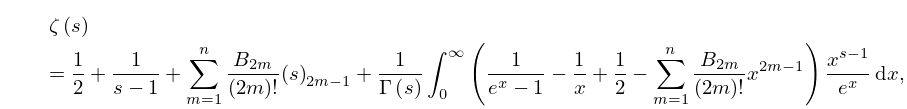
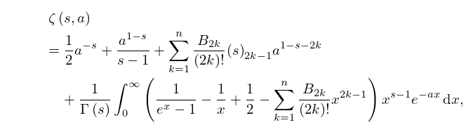
Derivable from (25.11.27) by adding and subtracting ${\sum }_{k=1}^n{B}_{2k}{x}^{2k-1}/(2k)!$ in the integrand, using (5.2.1), (5.2.5), and recognizing that ${({\mathrm{e}}^x-1)}^{-1}-x^{-1}+1/2-{\sum }_{k=1}^n{B}_{2k}{x}^{2k-1}/(2k)!=O\left(x^{2n+1}\right)$ as $x\to 0$, demonstrating the region of convergence.

Referenced by:

Erratum (V1.0.9) for Chapters 7, 25

Permalink:

http://dlmf.nist.gov/25.11.E28

Encodings:

pMML, png, TeX

Notational Change (effective with 1.0.9):

We have rewritten the original summation ${\sum }_{k=1}^n\frac{\mathrm{\Gamma }\left(s+2k-1\right)}{\mathrm{\Gamma }\left(s\right)}\frac{B_{2k}}{(2k)!}{a}^{-2k-s+1}$ more concisely as ${\sum }_{k=1}^n\frac{B_{2k}}{(2k)!}{\left(s\right)}_{2k-1}{a}^{1-s-2k}$ using the Pochhammer symbol.

See also:

Annotations for §25.11(vii), §25.11 and Ch.25

… ►where the integration contour is a loop around the negative real axis as described for (25.5.20). … ►

25.11.43 $$\zeta (s,a)-\frac{a^{1-s}}{s-1}-\frac{1}{2}{a}^{-s}\sim \sum _{k=1}^{\mathrm{\infty }}\frac{B_{2k}}{(2k)!}{\left(s\right)}_{2k-1}{a}^{1-s-2k}.$$

ⓘ

Symbols:

$B_n$: Bernoulli numbers, $\mathrm{\Gamma }\left(z\right)$: gamma function, $\zeta (s,a)$: Hurwitz zeta function, ${\left(a\right)}_n$: Pochhammer’s symbol (or shifted factorial), $\sim$: Poincaré asymptotic expansion, $!$: factorial (as in $n!$), $k$: nonnegative integer, $a$: real or complex parameter and $s$: complex variable

Keywords:

asymptotic approximation

Source:

Paris (2005b, (1.3), (1.4), p. 298)

Referenced by:

§25.11(xii), Erratum (V1.0.9) for Chapters 7, 25

Permalink:

http://dlmf.nist.gov/25.11.E43

Encodings:

pMML, png, TeX

Notational Change (effective with 1.0.9):

We have rewritten the original summation ${\sum }_{k=1}^{\mathrm{\infty }}\frac{B_{2k}}{(2k)!}\frac{\mathrm{\Gamma }\left(s+2k-1\right)}{\mathrm{\Gamma }\left(s\right)}{a}^{1-s-2k}$ more concisely as ${\sum }_{k=1}^{\mathrm{\infty }}\frac{B_{2k}}{(2k)!}{\left(s\right)}_{2k-1}{a}^{1-s-2k}$ using the Pochhammer symbol.

See also:

Annotations for §25.11(xii), §25.11 and Ch.25

…

17: 8 Incomplete Gamma and Related
Functions

…

18: 28 Mathieu Functions and Hill’s Equation

…

19: Errata

… ►

17.11.2 $${\mathrm{\Phi }}^{(2)}(a;b,b^{\prime };c,c^{\prime };q;x,y)=\frac{{(b,ax;q)}_{\mathrm{\infty }}}{{(c,x;q)}_{\mathrm{\infty }}}\sum _{n,r\geqq 0}\frac{{(a,b^{\prime };q)}_n{(c/b,x;q)}_r{b}^r{y}^n}{{(q,c^{\prime };q)}_n{(q;q)}_r{(ax;q)}_{n+r}}$$

The factor ${\left(q\right)}_r$ originally used in the denominator has been corrected to be ${(q;q)}_r$.

… ►

Pochhammer and $q$-Pochhammer symbols in several equations now correctly link to their definitions.

… ►

A sentence was added recommending §27.14(ii) for properties of ${(q;q)}_{\mathrm{\infty }}$.

… ►

Several new equations have been added. See (8.17.24), (20.7.34), §20.11(v), (26.12.27), (36.2.28), and (36.2.29).

… ►

Bibliographic citations were added in §§1.13(v), 10.14, 10.21(ii), 18.15(v), 18.32, 30.16(iii), 32.13(ii), and as general references in Chapters 19, 20, 22, and 23.

…

20: 5.11 Asymptotic Expansions

… ►

5.11.5 $$g_k=\sqrt{2}{\left(\frac{1}{2}\right)}_k{a}_{2k},$$

ⓘ

Symbols:

${\left(a\right)}_n$: Pochhammer’s symbol (or shifted factorial), $k$: nonnegative integer, $g_k$: coefficients and $a_k$: coefficient

Referenced by:

§5.11(i)

Permalink:

http://dlmf.nist.gov/5.11.E5

Encodings:

pMML, png, TeX

See also:

Annotations for §5.11(i), §5.11 and Ch.5

… ►Wrench (1968) gives exact values of $g_k$ up to $g_{20}$. … ►

5.11.19 $$\frac{\mathrm{\Gamma }\left(z+a\right)\mathrm{\Gamma }\left(z+b\right)}{\mathrm{\Gamma }\left(z+c\right)}\sim \sum _{k=0}^{\mathrm{\infty }}{(-1)}^k\frac{{\left(c-a\right)}_k{\left(c-b\right)}_k}{k!}\mathrm{\Gamma }\left(a+b-c+z-k\right).$$

ⓘ

Symbols:

$\mathrm{\Gamma }\left(z\right)$: gamma function, ${\left(a\right)}_n$: Pochhammer’s symbol (or shifted factorial), $\sim$: Poincaré asymptotic expansion, $!$: factorial (as in $n!$), $k$: nonnegative integer, $z$: complex variable, $a$: real or complex variable and $b$: real or complex variable

Referenced by:

§5.11(i), §5.11(iii)

Permalink:

http://dlmf.nist.gov/5.11.E19

Encodings:

pMML, png, TeX

See also:

Annotations for §5.11(iii), §5.11 and Ch.5

…