Olver hypergeometric function

SearchAdvancedHelp

(0.011 seconds)

31—40 of 69 matching pages

31: 13.23 Integrals

… ►

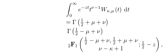
13.23.4 $${\int }_0^{\mathrm{\infty }}{\mathrm{e}}^{-zt}{t}^{\nu -1}{W}_{\kappa ,\mu }\left(t\right)dt=\mathrm{\Gamma }\left(\frac{1}{2}+\mu +\nu \right)\mathrm{\Gamma }\left(\frac{1}{2}-\mu +\nu \right){}_2{}^{}𝐅_1^{}(\genfrac{}{}{0pt}{}{\frac{1}{2}-\mu +\nu ,\frac{1}{2}+\mu +\nu }{\nu -\kappa +1};\frac{1}{2}-z),$$ $\mathrm{\Re }\left(\nu +\frac{1}{2}\right)>|\mathrm{\Re }\mu |$, $\mathrm{\Re }z>-\frac{1}{2}$,

ⓘ

Symbols:

$\mathrm{\Gamma }\left(z\right)$: gamma function, $W_{\kappa ,\mu }\left(z\right)$: Whittaker confluent hypergeometric function, $dx$: differential of $x$ , $\mathrm{e}$: base of natural logarithm, ${}_p{}^{}𝐅_q^{}(𝐚;𝐛;z)$ or ${}_p{}^{}𝐅_q^{}(\genfrac{}{}{0pt}{}{𝐚}{𝐛};z)$: scaled (or Olver’s) generalized hypergeometric function, $\int$: integral, $\mathrm{\Re }$: real part and $z$: complex variable

Keywords:

Laplace transform, Mellin transform

Referenced by:

§13.23(i)

Permalink:

http://dlmf.nist.gov/13.23.E4

Encodings:

pMML, png, TeX

See also:

Annotations for §13.23(i), §13.23 and Ch.13

…

32: Errata

… ►

The Olver hypergeometric function $𝐅(a,b;c;z)$, previously omitted from the left-hand sides to make the formulas more concise, has been added. In Equations (15.6.1)–(15.6.5), (15.6.7)–(15.6.9), the constraint has been added. In (15.6.6), the constraint has been added. In Section 15.6 Integral Representations, the sentence immediately following (15.6.9), “These representations are valid when , except (15.6.6) which holds for .”, has been removed.

…

33: 14.21 Definitions and Basic Properties

… ►Standard solutions: the associated Legendre functions $P_{\nu }^{\mu }\left(z\right)$, $P_{\nu }^{-\mu }\left(z\right)$, ${𝑸}_{\nu }^{\mu }\left(z\right)$, and ${𝑸}_{-\nu -1}^{\mu }\left(z\right)$. $P_{\nu }^{\pm \mu }\left(z\right)$ and ${𝑸}_{\nu }^{\mu }\left(z\right)$ exist for all values of $\nu$, $\mu$, and $z$, except possibly $z=\pm 1$ and $\mathrm{\infty }$, which are branch points (or poles) of the functions, in general. … … ►

§14.21(iii) Properties

… ►This includes, for example, the Wronskian relations (14.2.7)–(14.2.11); hypergeometric representations (14.3.6)–(14.3.10) and (14.3.15)–(14.3.20); results for integer orders (14.6.3)–(14.6.5), (14.6.7), (14.6.8), (14.7.6), (14.7.7), and (14.7.11)–(14.7.16); behavior at singularities (14.8.7)–(14.8.16); connection formulas (14.9.11)–(14.9.16); recurrence relations (14.10.3)–(14.10.7). …

34: 13.29 Methods of Computation

… ►However, this accuracy can be increased considerably by use of the exponentially-improved forms of expansion supplied by the combination of (13.7.10) and (13.7.11), or by use of the hyperasymptotic expansions given in Olde Daalhuis and Olver (1995a). … ►For $M(a,b,z)$ and $M_{\kappa ,\mu }\left(z\right)$ this means that in the sector $|\mathrm{ph}z|\le \pi$ we may integrate along outward rays from the origin with initial values obtained from (13.2.2) and (13.14.2). ►For $U(a,b,z)$ and $W_{\kappa ,\mu }\left(z\right)$ we may integrate along outward rays from the origin in the sectors , with initial values obtained from connection formulas in §13.2(vii), §13.14(vii). … ►The recurrence relations in §§13.3(i) and 13.15(i) can be used to compute the confluent hypergeometric functions in an efficient way. In the following two examples Olver’s algorithm (§3.6(v)) can be used. …

35: 13 Confluent Hypergeometric Functions

Chapter 13 Confluent Hypergeometric Functions

…

36: Frank W. J. Olver

Profile
Frank W. J. Olver

… ►Frank W. J. Olver (b. … ►Olver was an applied mathematician of world renown, one of the most widely recognized contemporary scholars in the field of special functions. …, Bessel functions, hypergeometric functions, Legendre functions). … ►In April 2011, NIST co-organized a conference on “Special Functions in the 21st Century: Theory & Application” which was dedicated to Olver. …

37: 15 Hypergeometric Function

Chapter 15 Hypergeometric Function

…

38: Bibliography Z

… ►

Numerical analysis of Struve functions with applications to other special functions. Ann. Numer. Math. 2 (1-4), pp. 199–208.

ⓘ

External Links:

ISSN 1021-2655, MathReview (F. W. J. Olver), ZentralBlatt

Referenced by:

§11.7(ii).

Encodings:

BibTeX

►

Distribution of zeros of Gauss and Kummer hypergeometric functions. A semiclassical approach. Ann. Numer. Math. 2 (1-4), pp. 457–472.

ⓘ

External Links:

ISSN 1021-2655, MathReview (B. D. Agrawal), ZentralBlatt

Referenced by:

§13.9(i), §15.13.

Encodings:

BibTeX

… ►

Doron Zeilberger’s Maple Packages and Programs Department of Mathematics, Rutgers University, New Jersey.

ⓘ

Notes:

Includes hypergeometric and $q$-hypergeometric summation, solution of difference equations (for example, by Petkovšek’s algorithm), combinatorial algorithms, and (package LUC) evaluation of zonal polynomials.

External Links:

Home Page

Referenced by:

§ ‣ Software Cross Index, § ‣ Software Cross Index, L. Lapointe and L. Vinet (1996).

Encodings:

BibTeX

… ►

The summation of series of hyperbolic functions. SIAM J. Math. Anal. 10 (1), pp. 192–206.

ⓘ

External Links:

ISSN 0036-1410, Document, MathReview (Y. L. Luke), ZentralBlatt

Referenced by:

§4.41.

Encodings:

BibTeX

… ►

Tablitsy vyrozhdennoi gipergeometricheskoi funktsii. Vyčisl. Centr Akad. Nauk SSSR, Moscow (Russian).

ⓘ

Notes:

Translated title: Tables of the confluent hypergeometric function

External Links:

MathReview (A. H. Stroud), ZentralBlatt

Referenced by:

1st item.

Encodings:

BibTeX

39: Bibliography T

… ►

Uniform asymptotic expansions of confluent hypergeometric functions. J. Inst. Math. Appl. 22 (2), pp. 215–223.

ⓘ

External Links:

ISSN 0020-2932, Document, MathReview (F. W. J. Olver), ZentralBlatt

Referenced by:

§13.8(ii), §13.8(ii).

Encodings:

BibTeX

…

40: 13.22 Zeros

§13.22 Zeros

►From (13.14.2) and (13.14.3) $M_{\kappa ,\mu }\left(z\right)$ has the same zeros as $M(\frac{1}{2}+\mu -\kappa ,1+2\mu ,z)$ and $W_{\kappa ,\mu }\left(z\right)$ has the same zeros as $U(\frac{1}{2}+\mu -\kappa ,1+2\mu ,z)$, hence the results given in §13.9 can be adopted. … ►For example, if $\mu (\ge 0)$ is fixed and $\kappa (>0)$ is large, then the $r$th positive zero ${\varphi }_r$ of $M_{\kappa ,\mu }\left(z\right)$ is given by …where $j_{2\mu ,r}$ is the $r$th positive zero of the Bessel function $J_{2\mu }\left(x\right)$ (§10.21(i)). …