Lebesgue%20constants

SearchAdvancedHelp

(0.002 seconds)

11—20 of 499 matching pages

11: 5.22 Tables

… ►Abramowitz and Stegun (1964, Chapter 6) tabulates $\mathrm{\Gamma }\left(x\right)$, $\ln \mathrm{\Gamma }\left(x\right)$, $\psi \left(x\right)$, and ${\psi }^{\prime }\left(x\right)$ for $x=1(.005)2$ to 10D; ${\psi }^{\prime \prime }\left(x\right)$ and ${\psi }^{(3)}\left(x\right)$ for $x=1(.01)2$ to 10D; $\mathrm{\Gamma }\left(n\right)$, $1/\mathrm{\Gamma }\left(n\right)$, $\mathrm{\Gamma }\left(n+\frac{1}{2}\right)$, $\psi \left(n\right)$, ${\log }_{10}\mathrm{\Gamma }\left(n\right)$, ${\log }_{10}\mathrm{\Gamma }\left(n+\frac{1}{3}\right)$, ${\log }_{10}\mathrm{\Gamma }\left(n+\frac{1}{2}\right)$, and ${\log }_{10}\mathrm{\Gamma }\left(n+\frac{2}{3}\right)$ for $n=1(1)101$ to 8–11S; $\mathrm{\Gamma }\left(n+1\right)$ for $n=100(100)1000$ to 20S. Zhang and Jin (1996, pp. 67–69 and 72) tabulates $\mathrm{\Gamma }\left(x\right)$, $1/\mathrm{\Gamma }\left(x\right)$, $\mathrm{\Gamma }\left(-x\right)$, $\ln \mathrm{\Gamma }\left(x\right)$, $\psi \left(x\right)$, $\psi \left(-x\right)$, ${\psi }^{\prime }\left(x\right)$, and ${\psi }^{\prime }\left(-x\right)$ for $x=0(.1)5$ to 8D or 8S; $\mathrm{\Gamma }\left(n+1\right)$ for $n=0(1)100(10)250(50)500(100)3000$ to 51S. … ►Abramov (1960) tabulates $\ln \mathrm{\Gamma }\left(x+\mathrm{i}y\right)$ for $x=1$ ($.01$) $2$, $y=0$ ($.01$) $4$ to 6D. Abramowitz and Stegun (1964, Chapter 6) tabulates $\ln \mathrm{\Gamma }\left(x+\mathrm{i}y\right)$ for $x=1$ ($.1$) $2$, $y=0$ ($.1$) $10$ to 12D. …Zhang and Jin (1996, pp. 70, 71, and 73) tabulates the real and imaginary parts of $\mathrm{\Gamma }\left(x+\mathrm{i}y\right)$, $\ln \mathrm{\Gamma }\left(x+\mathrm{i}y\right)$, and $\psi \left(x+\mathrm{i}y\right)$ for $x=0.5,1,5,10$, $y=0(.5)10$ to 8S.

12: 18.2 General Orthogonal Polynomials

… ►More generally than (18.2.1)–(18.2.3), $w(x)dx$ may be replaced in (18.2.1) by $d\mu (x)$, where the measure $\mu$ is the Lebesgue–Stieltjes measure ${\mu }_{\alpha }$ corresponding to a bounded nondecreasing function $\alpha$ on the closure of $(a,b)$ with an infinite number of points of increase, and such that for all $n$. … ►

§18.2(iii) Standardization and Related Constants

… ►

Constants

… ►(i) the traditional OP standardizations of Table 18.3.1, where each is defined in terms of the above constants. … ►, of the form $w(x)dx$) nor is it necessarily unique, up to a positive constant factor. …

13: 2.4 Contour Integrals

… ►Then … … ►Then the Laplace transform …where $\sigma$ ($\ge c$) is a constant. … ►If this integral converges uniformly at each limit for all sufficiently large $t$, then by the Riemann–Lebesgue lemma (§1.8(i)) …

14: 18.18 Sums

… ►

18.18.1 $$a_n=\frac{n!(2n+\alpha +\beta +1)\mathrm{\Gamma }\left(n+\alpha +\beta +1\right)}{2^{\alpha +\beta +1}\mathrm{\Gamma }\left(n+\alpha +1\right)\mathrm{\Gamma }\left(n+\beta +1\right)}{\int }_{-1}^{1}f(x)P_n^{(\alpha ,\beta )}\left(x\right){(1-x)}^{\alpha }{(1+x)}^{\beta }dx.$$

ⓘ

Defines:

$a_n$ (locally)

Symbols:

$\mathrm{\Gamma }\left(z\right)$: gamma function, $P_n^{(\alpha ,\beta )}\left(x\right)$: Jacobi polynomial, $dx$: differential of $x$ , $!$: factorial (as in $n!$), $\int$: integral, $n$: nonnegative integer, $f(z)$: analytic function and $x$: real variable

Referenced by:

§18.18(i), §18.18(i)

Permalink:

http://dlmf.nist.gov/18.18.E1

Encodings:

pMML, png, TeX

See also:

Annotations for §18.18(i), §18.18(i), §18.18 and Ch.18

… ►

18.18.5 $$b_n=\frac{n!}{\mathrm{\Gamma }\left(n+\alpha +1\right)}{\int }_0^{\mathrm{\infty }}f(x)L_n^{(\alpha )}\left(x\right){\mathrm{e}}^{-x}{x}^{\alpha }dx.$$

ⓘ

Symbols:

$\mathrm{\Gamma }\left(z\right)$: gamma function, $L_n^{(\alpha )}\left(x\right)$: Laguerre (or generalized Laguerre) polynomial, $dx$: differential of $x$ , $\mathrm{e}$: base of natural logarithm, $!$: factorial (as in $n!$), $\int$: integral, $n$: nonnegative integer, $f(z)$: analytic function and $x$: real variable

Referenced by:

§18.18(i)

Permalink:

http://dlmf.nist.gov/18.18.E5

Encodings:

pMML, png, TeX

See also:

Annotations for §18.18(i), §18.18(i), §18.18 and Ch.18

… ►

Expansion of $L^2$ functions

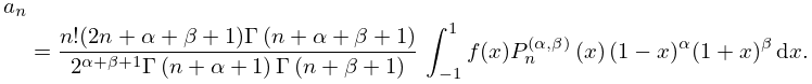
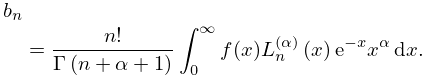
►In all three cases of Jacobi, Laguerre and Hermite, if $f(x)$ is $L^2$ on the corresponding interval with respect to the corresponding weight function and if $a_n,b_n,d_n$ are given by (18.18.1), (18.18.5), (18.18.7), respectively, then the respective series expansions (18.18.2), (18.18.4), (18.18.6) are valid with the sums converging in $L^2$ sense. … ►See Andrews et al. (1999, Lemma 7.1.1) for the more general expansion of $P_n^{(\gamma ,\delta )}\left(x\right)$ in terms of $P_n^{(\alpha ,\beta )}\left(x\right)$. …

15: 1.16 Distributions

… ►where ${\alpha }_1$ and ${\alpha }_2$ are real or complex constants. … ►, a function $f$ on $I$ which is absolutely Lebesgue integrable on every compact subset of $I$) such that …More generally, for $\alpha :[a,b]\to [-\mathrm{\infty },\mathrm{\infty }]$ a nondecreasing function the corresponding Lebesgue–Stieltjes measure ${\mu }_{\alpha }$ (see §1.4(v)) can be considered as a distribution: … ►where $c$ is a constant. … ►Since ${\delta }_{x_0}$ is the Lebesgue–Stieltjes measure ${\mu }_{\alpha }$ corresponding to $\alpha (x)=H\left(x-x_0\right)$ (see §1.4(v)), formula (1.16.16) is a special case of (1.16.3_5), (1.16.9_5) for that choice of $\alpha$. …

16: 25.12 Polylogarithms

… ►

►►

Figure 25.12.1: Dilogarithm function ${\mathrm{Li}}_2\left(x\right)$, Magnify

►

►

►

Figure 25.12.2: Absolute value of the dilogarithm function $\left|{\mathrm{Li}}_2\left(x+\mathrm{i}y\right)\right|$, $-20\le x\le 20$, $-20\le y\le 20$. … Magnify 3D Help

… ►

25.12.11 $${\mathrm{Li}}_s\left(z\right)\equiv \frac{z}{\mathrm{\Gamma }\left(s\right)}{\int }_0^{\mathrm{\infty }}\frac{x^{s-1}}{{\mathrm{e}}^x-z}dx,$$

ⓘ

Symbols:

$\mathrm{\Gamma }\left(z\right)$: gamma function, $dx$: differential of $x$ , $\equiv$: equals by definition, $\mathrm{e}$: base of natural logarithm, $\int$: integral, ${\mathrm{Li}}_s\left(z\right)$: polylogarithm, $x$: real variable, $s$: complex variable and $z$: complex variable

Keywords:

improper integral, integral representation

Source:

Lewin (1981, (7.188), p. 236)

Referenced by:

(25.12.16), §25.12(ii)

Permalink:

http://dlmf.nist.gov/25.12.E11

Encodings:

pMML, png, TeX

See also:

Annotations for §25.12(ii), §25.12(ii), §25.12 and Ch.25

… ►

25.12.14 $$F_s(x)=\frac{1}{\mathrm{\Gamma }\left(s+1\right)}{\int }_0^{\mathrm{\infty }}\frac{t^s}{{\mathrm{e}}^{t-x}+1}dt,$$ $s>-1$,

ⓘ

Defines:

$F_s(x)$: Fermi–Dirac integral (locally)

Symbols:

$\mathrm{\Gamma }\left(z\right)$: gamma function, $dx$: differential of $x$ , $\mathrm{e}$: base of natural logarithm, $\int$: integral, $x$: real variable and $s$: complex variable

Keywords:

definition, Fermi–Dirac integral, improper integral, integral representation

Source:

Dingle (1957b, (1), p. 226)

Referenced by:

(25.12.16), 3rd item, 5th item

Permalink:

http://dlmf.nist.gov/25.12.E14

Encodings:

pMML, png, TeX

See also:

Annotations for §25.12(iii), §25.12 and Ch.25

… ►Sometimes the factor $1/\mathrm{\Gamma }\left(s+1\right)$ is omitted. …

17: 2.10 Sums and Sequences

… ►Formula (2.10.2) is useful for evaluating the constant term in expansions obtained from (2.10.1). …where $\gamma$ is Euler’s constant (§5.2(ii)) and ${\zeta }^{\prime }$ is the derivative of the Riemann zeta function (§25.2(i)). ${\mathrm{e}}^C$ is sometimes called Glaisher’s constant. … ►where $\alpha$ ($\ne -1$) is a real constant, and … ►Hence by the Riemann–Lebesgue lemma (§1.8(i)) …

18: 32.8 Rational Solutions

… ►with $\kappa$, $\lambda$, and $\mu$ arbitrary constants. ►In the general case assume $\gamma \delta \ne 0$, so that as in §32.2(ii) we may set $\gamma =1$ and $\delta =-1$. … ►with $\kappa$ and $\mu$ arbitrary constants. … ►

$\alpha =\frac{1}{2}{a}^2$, $\beta =-\frac{1}{2}{(a+n)}^2$, and $\gamma =m$, with $m+n$ even.

… ►with $\kappa$ and $\mu$ arbitrary constants. …

19: 25.20 Approximations

… ►

Cody et al. (1971) gives rational approximations for $\zeta \left(s\right)$ in the form of quotients of polynomials or quotients of Chebyshev series. The ranges covered are $0.5\le s\le 5$, $5\le s\le 11$, $11\le s\le 25$, $25\le s\le 55$. Precision is varied, with a maximum of 20S.

… ►

Antia (1993) gives minimax rational approximations for $\mathrm{\Gamma }\left(s+1\right)F_s(x)$, where $F_s(x)$ is the Fermi–Dirac integral (25.12.14), for the intervals and , with $s=-\frac{1}{2},\frac{1}{2},\frac{3}{2},\frac{5}{2}$. For each $s$ there are three sets of approximations, with relative maximum errors ${10}^{-4},{10}^{-8},{10}^{-12}$.

20: 30.9 Asymptotic Approximations and Expansions

… ►

§30.9(i) Prolate Spheroidal Wave Functions

►As ${\gamma }^2\to +\mathrm{\infty }$, with $q=2(n-m)+1$, … ►The asymptotic behavior of ${\lambda }_n^m\left({\gamma }^2\right)$ and $a_{n,k}^m({\gamma }^2)$ as $n\to \mathrm{\infty }$ in descending powers of $2n+1$ is derived in Meixner (1944). …The asymptotic behavior of ${\mathrm{𝖯𝗌}}_n^m(x,{\gamma }^2)$ and ${\mathrm{𝖰𝗌}}_n^m(x,{\gamma }^2)$ as $x\to \pm 1$ is given in Erdélyi et al. (1955, p. 151). The behavior of ${\lambda }_n^m\left({\gamma }^2\right)$ for complex ${\gamma }^2$ and large $|{\lambda }_n^m\left({\gamma }^2\right)|$ is investigated in Hunter and Guerrieri (1982). …