Laplace transform with respect to lattice parameter

SearchAdvancedHelp

(0.003 seconds)

21—30 of 910 matching pages

21: 13.10 Integrals

… ►

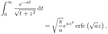
§13.10(ii) Laplace Transforms

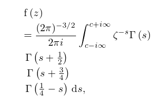
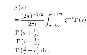
… ►For additional Laplace transforms see Erdélyi et al. (1954a, §§4.22, 5.20), Oberhettinger and Badii (1973, §1.17), and Prudnikov et al. (1992a, §§3.34, 3.35). Inverse Laplace transforms are given in Oberhettinger and Badii (1973, §2.16) and Prudnikov et al. (1992b, §§3.33, 3.34). ►

§13.10(iii) Mellin Transforms

… ►

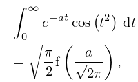
§13.10(iv) Fourier Transforms

…

22: Bibliography D

… ►

Integral Transforms and their Applications. 2nd edition, Applied Mathematical Sciences, Vol. 25, Springer-Verlag, New York.

ⓘ

External Links:

ISBN 0-387-96080-5, MathReview, ZentralBlatt

Referenced by:

§1.14(vii).

Encodings:

BibTeX

… ►

Integral transforms and their applications. Third edition, CRC Press, Boca Raton, FL.

ⓘ

External Links:

ISBN 978-1-4822-2357-6, MathReview Entry, ZentralBlatt

Referenced by:

§1.16(viii).

Encodings:

BibTeX

… ►

Strong asymptotics of orthogonal polynomials with respect to exponential weights. Comm. Pure Appl. Math. 52 (12), pp. 1491–1552.

ⓘ

External Links:

ISSN 0010-3640, Document, MathReview (D. S. Lubinsky), ZentralBlatt

Referenced by:

§18.32.

Encodings:

BibTeX

►

Uniform asymptotics for polynomials orthogonal with respect to varying exponential weights and applications to universality questions in random matrix theory. Comm. Pure Appl. Math. 52 (11), pp. 1335–1425.

ⓘ

External Links:

ISSN 0010-3640, Document, MathReview (D. S. Lubinsky), ZentralBlatt

Referenced by:

§18.32.

Encodings:

BibTeX

… ►

Handbuch der Laplace-Transformation. Bd. II. Anwendungen der Laplace-Transformation. 1. Abteilung. Birkhäuser Verlag, Basel und Stuttgart (German).

ⓘ

External Links:

MathReview (I. I. Hirschman), ZentralBlatt

Referenced by:

§2.5(i).

Encodings:

BibTeX

…

23: 24.13 Integrals

… ►

§24.13(iii) Compendia

►For Laplace and inverse Laplace transforms see Prudnikov et al. (1992a, §§3.28.1–3.28.2) and Prudnikov et al. (1992b, §§3.26.1–3.26.2). …

24: 12.16 Mathematical Applications

… ►PCFs are also used in integral transforms with respect to the parameter, and inversion formulas exist for kernels containing PCFs. …Integral transforms and sampling expansions are considered in Jerri (1982).

25: 18.17 Integrals

… ►

§18.17(vi) Laplace Transforms

►Many of the Fourier transforms given in §18.17(v) have analytic continuations to Laplace transforms. … ►

Jacobi

… ►

Laguerre

… ►

Hermite

…

26: 10.73 Physical Applications

… ►Bessel functions of the first kind, $J_n\left(x\right)$, arise naturally in applications having cylindrical symmetry in which the physics is described either by Laplace’s equation ${\nabla }^{2}V=0$, or by the Helmholtz equation $({\nabla }^2+k^2)\psi =0$. ►Laplace’s equation governs problems in heat conduction, in the distribution of potential in an electrostatic field, and in hydrodynamics in the irrotational motion of an incompressible fluid. … … ►The analysis of the current distribution in circular conductors leads to the Kelvin functions $\mathrm{ber}x$, $\mathrm{bei}x$, $\ker x$, and $\mathrm{kei}x$. …

27: Bibliography S

… ►

Orthogonal polynomials arising in the numerical evaluation of inverse Laplace transforms. Math. Tables Aids Comput. 9 (52), pp. 164–177.

ⓘ

External Links:

FullText, MathReview (S. C. van Veen), ZentralBlatt

Referenced by:

§3.5(viii).

Encodings:

BibTeX

… ►

The Laplace Transform: Theory and Applications. Undergraduate Texts in Mathematics, Springer-Verlag, New York.

ⓘ

External Links:

ISBN 0-387-98698-7, MathReview (Philip Heywood), ZentralBlatt

Referenced by:

§1.14(iii), §1.14(vii).

Encodings:

BibTeX

… ►

Numerical evaluation of spherical Bessel transforms via fast Fourier transforms. J. Comput. Phys. 100 (2), pp. 294–296.

ⓘ

External Links:

ISSN 0021-9991, Document, MathReview, ZentralBlatt

Referenced by:

§10.74(vii).

Encodings:

BibTeX

… ►

The Laplace transforms of products of Airy functions. Dirāsāt Ser. B Pure Appl. Sci. 19 (2), pp. 7–11.

ⓘ

External Links:

ISSN 0253-424X, MathReview

Referenced by:

§9.10(v).

Encodings:

BibTeX

… ►

A Guide to Distribution Theory and Fourier Transforms. Studies in Advanced Mathematics, CRC Press, Boca Raton, FL.

ⓘ

External Links:

ISBN 0-8493-8273-4, MathReview (J. Horváth), ZentralBlatt

Referenced by:

§18.17(v).

Encodings:

BibTeX

…

28: 7.7 Integral Representations

… ►

7.7.4 $${\int }_0^{\mathrm{\infty }}\frac{{\mathrm{e}}^{-at}}{\sqrt{t+z^2}}dt=\sqrt{\frac{\pi }{a}}{\mathrm{e}}^{a{z}^2}\mathrm{erfc}\left(\sqrt{a}z\right),$$ $\mathrm{\Re }a>0$, $\mathrm{\Re }z>0$.

ⓘ

Symbols:

$\pi$: the ratio of the circumference of a circle to its diameter, $\mathrm{erfc}z$: complementary error function, $dx$: differential of $x$ , $\mathrm{e}$: base of natural logarithm, $\int$: integral, $\mathrm{\Re }$: real part and $z$: complex variable

Keywords:

Laplacetransform

A&S Ref:

7.4.8

Referenced by:

§7.7(i)

Permalink:

http://dlmf.nist.gov/7.7.E4

Encodings:

pMML, png, TeX

See also:

Annotations for §7.7(i), §7.7 and Ch.7

… ►

7.7.13 $$\mathrm{f}\left(z\right)=\frac{{(2\pi )}^{-3/2}}{2\pi \mathrm{i}}{\int }_{c-\mathrm{i}\mathrm{\infty }}^{c+\mathrm{i}\mathrm{\infty }}{\zeta }^{-s}\mathrm{\Gamma }\left(s\right)\mathrm{\Gamma }\left(s+\frac{1}{2}\right)\mathrm{\Gamma }\left(s+\frac{3}{4}\right)\mathrm{\Gamma }\left(\frac{1}{4}-s\right)ds,$$

ⓘ

Symbols:

$\mathrm{\Gamma }\left(z\right)$: gamma function, $\mathrm{f}\left(z\right)$: auxiliary function for Fresnel integrals, $\pi$: the ratio of the circumference of a circle to its diameter, $dx$: differential of $x$ , $\mathrm{i}$: imaginary unit, $\int$: integral, $z$: complex variable, $\zeta$: change of variable and $c$: constant

Keywords:

Mellin transform

Referenced by:

§7.7(ii), §7.7(ii)

Permalink:

http://dlmf.nist.gov/7.7.E13

Encodings:

pMML, png, TeX

See also:

Annotations for §7.7(ii), §7.7(ii), §7.7 and Ch.7

►

7.7.14 $$\mathrm{g}\left(z\right)=\frac{{(2\pi )}^{-3/2}}{2\pi \mathrm{i}}{\int }_{c-\mathrm{i}\mathrm{\infty }}^{c+\mathrm{i}\mathrm{\infty }}{\zeta }^{-s}\mathrm{\Gamma }\left(s\right)\mathrm{\Gamma }\left(s+\frac{1}{2}\right)\mathrm{\Gamma }\left(s+\frac{1}{4}\right)\mathrm{\Gamma }\left(\frac{3}{4}-s\right)ds.$$

ⓘ

Symbols:

$\mathrm{\Gamma }\left(z\right)$: gamma function, $\mathrm{g}\left(z\right)$: auxiliary function for Fresnel integrals, $\pi$: the ratio of the circumference of a circle to its diameter, $dx$: differential of $x$ , $\mathrm{i}$: imaginary unit, $\int$: integral, $z$: complex variable, $\zeta$: change of variable and $c$: constant

Keywords:

Mellin transform

Referenced by:

§7.7(ii), §7.7(ii)

Permalink:

http://dlmf.nist.gov/7.7.E14

Encodings:

pMML, png, TeX

See also:

Annotations for §7.7(ii), §7.7(ii), §7.7 and Ch.7

… ►

7.7.15 $${\int }_0^{\mathrm{\infty }}{\mathrm{e}}^{-at}\cos \left(t^2\right)dt=\sqrt{\frac{\pi }{2}}\mathrm{f}\left(\frac{a}{\sqrt{2\pi }}\right),$$ $\mathrm{\Re }a>0$,

ⓘ

Symbols:

$\mathrm{f}\left(z\right)$: auxiliary function for Fresnel integrals, $\pi$: the ratio of the circumference of a circle to its diameter, $\cos z$: cosine function, $dx$: differential of $x$ , $\mathrm{e}$: base of natural logarithm, $\int$: integral and $\mathrm{\Re }$: real part

Keywords:

Laplacetransform

A&S Ref:

7.4.22 (in different notation)

Referenced by:

§7.14(ii)

Permalink:

http://dlmf.nist.gov/7.7.E15

Encodings:

pMML, png, TeX

See also:

Annotations for §7.7(ii), §7.7(ii), §7.7 and Ch.7

►

7.7.16 $${\int }_0^{\mathrm{\infty }}{\mathrm{e}}^{-at}\sin \left(t^2\right)dt=\sqrt{\frac{\pi }{2}}\mathrm{g}\left(\frac{a}{\sqrt{2\pi }}\right),$$ $\mathrm{\Re }a>0$.

ⓘ

Symbols:

$\mathrm{g}\left(z\right)$: auxiliary function for Fresnel integrals, $\pi$: the ratio of the circumference of a circle to its diameter, $dx$: differential of $x$ , $\mathrm{e}$: base of natural logarithm, $\int$: integral, $\mathrm{\Re }$: real part and $\sin z$: sine function

Keywords:

Laplacetransform

A&S Ref:

7.4.23 (in different notation)

Referenced by:

§7.14(ii)

Permalink:

http://dlmf.nist.gov/7.7.E16

Encodings:

pMML, png, TeX

See also:

Annotations for §7.7(ii), §7.7(ii), §7.7 and Ch.7

…

29: 16.15 Integral Representations and Integrals

… ►

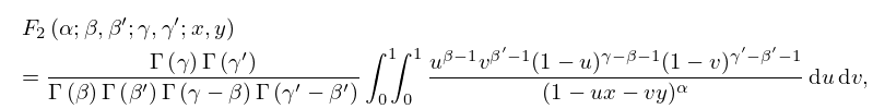
16.15.1 $$F_1(\alpha ;\beta ,{\beta }^{\prime };\gamma ;x,y)=\frac{\mathrm{\Gamma }\left(\gamma \right)}{\mathrm{\Gamma }\left(\alpha \right)\mathrm{\Gamma }\left(\gamma -\alpha \right)}{\int }_0^1\frac{u^{\alpha -1}{(1-u)}^{\gamma -\alpha -1}}{{(1-ux)}^{\beta }{(1-uy)}^{{\beta }^{\prime }}}du,$$ $\mathrm{\Re }\alpha >0$, $\mathrm{\Re }\left(\gamma -\alpha \right)>0$,

ⓘ

Symbols:

$F_1(\alpha ;\beta ,{\beta }^{\prime };\gamma ;x,y)$: first Appell function, $\mathrm{\Gamma }\left(z\right)$: gamma function, $dx$: differential of $x$ , $\int$: integral and $\mathrm{\Re }$: real part

Keywords:

Mellin transform

Permalink:

http://dlmf.nist.gov/16.15.E1

Encodings:

pMML, png, TeX

See also:

Annotations for §16.15 and Ch.16

►

16.15.2 $$F_2(\alpha ;\beta ,{\beta }^{\prime };\gamma ,{\gamma }^{\prime };x,y)=\frac{\mathrm{\Gamma }\left(\gamma \right)\mathrm{\Gamma }\left({\gamma }^{\prime }\right)}{\mathrm{\Gamma }\left(\beta \right)\mathrm{\Gamma }\left({\beta }^{\prime }\right)\mathrm{\Gamma }\left(\gamma -\beta \right)\mathrm{\Gamma }\left({\gamma }^{\prime }-{\beta }^{\prime }\right)}{\int }_0^1{\int }_0^1\frac{u^{\beta -1}{v}^{{\beta }^{\prime }-1}{(1-u)}^{\gamma -\beta -1}{(1-v)}^{{\gamma }^{\prime }-{\beta }^{\prime }-1}}{{(1-ux-vy)}^{\alpha }}dudv,$$ $\mathrm{\Re }\gamma >\mathrm{\Re }\beta >0$, $\mathrm{\Re }{\gamma }^{\prime }>\mathrm{\Re }{\beta }^{\prime }>0$,

ⓘ

Symbols:

$F_2(\alpha ;\beta ,{\beta }^{\prime };\gamma ,{\gamma }^{\prime };x,y)$: second Appell function, $\mathrm{\Gamma }\left(z\right)$: gamma function, $dx$: differential of $x$ , $\int$: integral and $\mathrm{\Re }$: real part

Keywords:

Mellin transform

Permalink:

http://dlmf.nist.gov/16.15.E2

Encodings:

pMML, png, TeX

See also:

Annotations for §16.15 and Ch.16

… ►These representations can be used to derive analytic continuations of the Appell functions, including convergent series expansions for large $x$, large $y$, or both. For inverse Laplace transforms of Appell functions see Prudnikov et al. (1992b, §3.40).

30: 8.19 Generalized Exponential Integral

… ►

§8.19(i) Definition and Integral Representations

… ►

8.19.2 $$E_p\left(z\right)=z^{p-1}{\int }_z^{\mathrm{\infty }}\frac{{\mathrm{e}}^{-t}}{t^p}dt.$$

ⓘ

Symbols:

$dx$: differential of $x$ , $\mathrm{e}$: base of natural logarithm, $E_p\left(z\right)$: generalized exponential integral, $\int$: integral, $z$: complex variable and $p$: parameter

Keywords:

Laplacetransform, Mellin transform

Referenced by:

§8.19(i), §8.19(viii)

Permalink:

http://dlmf.nist.gov/8.19.E2

Encodings:

pMML, png, TeX

See also:

Annotations for §8.19(i), §8.19 and Ch.8

… ►

8.19.3 $$E_p\left(z\right)={\int }_1^{\mathrm{\infty }}\frac{{\mathrm{e}}^{-zt}}{t^p}dt,$$ ,

ⓘ

Symbols:

$\pi$: the ratio of the circumference of a circle to its diameter, $dx$: differential of $x$ , $\mathrm{e}$: base of natural logarithm, $E_p\left(z\right)$: generalized exponential integral, $\int$: integral, $\mathrm{ph}$: phase, $z$: complex variable and $p$: parameter

Keywords:

Laplacetransform, Mellin transform

A&S Ref:

5.1.4

Referenced by:

§8.19(iii)

Permalink:

http://dlmf.nist.gov/8.19.E3

Encodings:

pMML, png, TeX

See also:

Annotations for §8.19(i), §8.19(i), §8.19 and Ch.8

… ►In Figures 8.19.2–8.19.5, height corresponds to the absolute value of the function and color to the phase. … ►

§8.19(vi) Relation to Confluent Hypergeometric Function

…