L orthornormal basis

SearchAdvancedHelp

(0.001 seconds)

21—30 of 113 matching pages

21: 11.4 Basic Properties

… ►

11.4.4 $${𝐋}_{-n-\frac{1}{2}}\left(z\right)=I_{n+\frac{1}{2}}\left(z\right).$$

ⓘ

Symbols:

$I_{\nu }\left(z\right)$: modified Bessel function of the first kind, ${𝐋}_{\nu }\left(z\right)$: modified Struve function, $z$: complex variable and $n$: integer order

A&S Ref:

12.2.10

Referenced by:

§11.4(i)

Permalink:

http://dlmf.nist.gov/11.4.E4

Encodings:

pMML, png, TeX

See also:

Annotations for §11.4(i), §11.4 and Ch.11

… ►

11.4.29 $$\frac{d}{dz}\left(z^{\nu }{𝐋}_{\nu }\left(z\right)\right)=z^{\nu }{𝐋}_{\nu -1}\left(z\right),$$

ⓘ

Symbols:

$\frac{df}{dx}$: derivative of $f$ with respect to $x$ , ${𝐋}_{\nu }\left(z\right)$: modified Struve function, $z$: complex variable and $\nu$: real or complex order

Referenced by:

§10.43(i)

Permalink:

http://dlmf.nist.gov/11.4.E29

Encodings:

pMML, png, TeX

See also:

Annotations for §11.4(v), §11.4 and Ch.11

… ►where ${\mathscr{H}}_{\nu }(z)$ denotes either ${𝐇}_{\nu }\left(z\right)$ or ${𝐋}_{\nu }\left(z\right)$. … ►

${𝐋}_0^{\prime }\left(z\right)={\displaystyle \frac{2}{\pi }}+{𝐋}_1\left(z\right),$

►

${\displaystyle \frac{d}{dz}}(z{𝐋}_1\left(z\right))=z{𝐋}_0\left(z\right).$

…

22: 25.19 Tables

… ►

Cloutman (1989) tabulates $\mathrm{\Gamma }\left(s+1\right)F_s(x)$, where $F_s(x)$ is the Fermi–Dirac integral (25.12.14), for $s=-\frac{1}{2},\frac{1}{2},\frac{3}{2},\frac{5}{2}$, $x=-5(.05)25$, to 12S.

►

Fletcher et al. (1962, §22.1) lists many sources for earlier tables of $\zeta \left(s\right)$ for both real and complex $s$. §22.133 gives sources for numerical values of coefficients in the Riemann–Siegel formula, §22.15 describes tables of values of $\zeta (s,a)$, and §22.17 lists tables for some Dirichlet $L$-functions for real characters. For tables of dilogarithms, polylogarithms, and Clausen’s integral see §§22.84–22.858.

23: 23.1 Special Notation

… ► ►►

$𝕃$	lattice in $ℂ$.
…

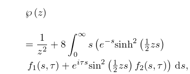
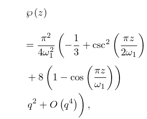
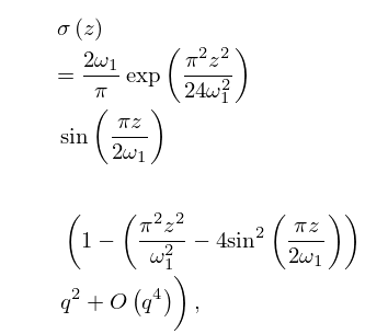
►The main functions treated in this chapter are the Weierstrass $\mathrm{\wp }$-function $\mathrm{\wp }\left(z\right)=\mathrm{\wp }\left(z|𝕃\right)=\mathrm{\wp }(z;g_2,g_3)$; the Weierstrass zeta function $\zeta \left(z\right)=\zeta \left(z|𝕃\right)=\zeta (z;g_2,g_3)$; the Weierstrass sigma function $\sigma \left(z\right)=\sigma \left(z|𝕃\right)=\sigma (z;g_2,g_3)$; the elliptic modular function $\lambda \left(\tau \right)$; Klein’s complete invariant $J\left(\tau \right)$; Dedekind’s eta function $\eta \left(\tau \right)$. …

24: 25.1 Special Notation

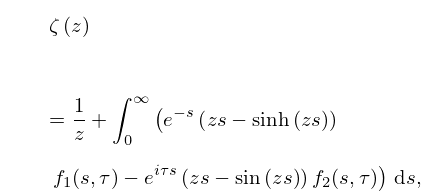
… ►The main related functions are the Hurwitz zeta function $\zeta (s,a)$, the dilogarithm ${\mathrm{Li}}_2\left(z\right)$, the polylogarithm ${\mathrm{Li}}_s\left(z\right)$ (also known as Jonquière’s function $\varphi (z,s)$), Lerch’s transcendent $\mathrm{\Phi }(z,s,a)$, and the Dirichlet $L$-functions $L(s,\chi )$.

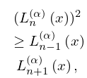
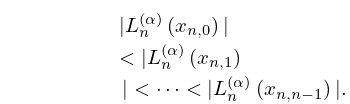
25: 18.14 Inequalities

… ►

18.14.8 $${\mathrm{e}}^{-\frac{1}{2}x}\left|L_n^{(\alpha )}\left(x\right)\right|\le L_n^{(\alpha )}\left(0\right)=\frac{{\left(\alpha +1\right)}_n}{n!},$$ , $\alpha \ge 0$.

ⓘ

Symbols:

$L_n^{(\alpha )}\left(x\right)$: Laguerre (or generalized Laguerre) polynomial, ${\left(a\right)}_n$: Pochhammer’s symbol (or shifted factorial), $\mathrm{e}$: base of natural logarithm, $!$: factorial (as in $n!$), $n$: nonnegative integer and $x$: real variable

Proved:

Koornwinder (1977, Remark 4.1)(proved)

Proof sketch:

The case $\alpha =0$ follows from the result on monotonic weight functions in §18.2(xii).

A&S Ref:

22.14.13

Referenced by:

§18.14(i), §18.2(xii)

Permalink:

http://dlmf.nist.gov/18.14.E8

Encodings:

pMML, png, TeX

See also:

Annotations for §18.14(i), §18.14(i), §18.14 and Ch.18

… ►

18.14.12 $${(L_n^{(\alpha )}\left(x\right))}^2\ge L_{n-1}^{(\alpha )}\left(x\right)L_{n+1}^{(\alpha )}\left(x\right),$$ , $\alpha \ge 0$.

ⓘ

Symbols:

$L_n^{(\alpha )}\left(x\right)$: Laguerre (or generalized Laguerre) polynomial, $n$: nonnegative integer and $x$: real variable

Referenced by:

§18.14(ii)

Permalink:

http://dlmf.nist.gov/18.14.E12

Encodings:

pMML, png, TeX

See also:

Annotations for §18.14(ii), §18.14(ii), §18.14 and Ch.18

… ►Let the maxima $x_{n,m}$, $m=0,1,\mathrm{\dots },n-1$, of $|L_n^{(\alpha )}\left(x\right)|$ in $[0,\mathrm{\infty })$ be arranged so that … ►

$|L_n^{(\alpha )}\left(x_{n,0}\right)|>|L_n^{(\alpha )}\left(x_{n,1}\right)|>\mathrm{\cdots }>|L_n^{(\alpha )}\left(x_{n,m}\right)|,$

… ►

18.14.24

ⓘ

Symbols:

$L_n^{(\alpha )}\left(x\right)$: Laguerre (or generalized Laguerre) polynomial, $n$: nonnegative integer and $x$: real variable

Referenced by:

§18.14(iii)

Permalink:

http://dlmf.nist.gov/18.14.E24

Encodings:

pMML, png, TeX

See also:

Annotations for §18.14(iii), §18.14(iii), §18.14 and Ch.18

…

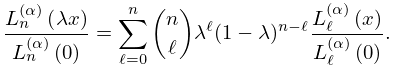
26: 18.18 Sums

… ►

Expansion of $L^2$ functions

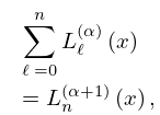
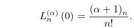
►In all three cases of Jacobi, Laguerre and Hermite, if $f(x)$ is $L^2$ on the corresponding interval with respect to the corresponding weight function and if $a_n,b_n,d_n$ are given by (18.18.1), (18.18.5), (18.18.7), respectively, then the respective series expansions (18.18.2), (18.18.4), (18.18.6) are valid with the sums converging in $L^2$ sense. … ►

18.18.10 $$L_n^{({\alpha }_1+\mathrm{\cdots }+{\alpha }_r+r-1)}\left(x_1+\mathrm{\cdots }+x_r\right)=\sum _{m_1+\mathrm{\cdots }+m_r=n}{L}_{m_1}^{({\alpha }_1)}\left(x_1\right)\mathrm{\cdots }{L}_{m_r}^{({\alpha }_r)}\left(x_r\right).$$

ⓘ

Symbols:

$L_n^{(\alpha )}\left(x\right)$: Laguerre (or generalized Laguerre) polynomial, $m$: nonnegative integer, $n$: nonnegative integer and $x$: real variable

Referenced by:

§18.18(ii), §18.18(viii)

Permalink:

http://dlmf.nist.gov/18.18.E10

Encodings:

pMML, png, TeX

See also:

Annotations for §18.18(ii), §18.18(ii), §18.18 and Ch.18

… ►

18.18.12 $$\frac{L_n^{(\alpha )}\left(\lambda x\right)}{L_n^{(\alpha )}\left(0\right)}=\sum _{\mathrm{\ell }=0}^n\left(\genfrac{}{}{0.0pt}{}{n}{\mathrm{\ell }}\right){\lambda }^{\mathrm{\ell }}{(1-\lambda )}^{n-\mathrm{\ell }}\frac{L_{\mathrm{\ell }}^{(\alpha )}\left(x\right)}{L_{\mathrm{\ell }}^{(\alpha )}\left(0\right)}.$$

ⓘ

Symbols:

$L_n^{(\alpha )}\left(x\right)$: Laguerre (or generalized Laguerre) polynomial, $\left(\genfrac{}{}{0.0pt}{}{m}{n}\right)$: binomial coefficient, $\mathrm{\ell }$: nonnegative integer, $n$: nonnegative integer and $x$: real variable

Referenced by:

(18.17.34_5), §18.18(iii), §18.18(iv)

Permalink:

http://dlmf.nist.gov/18.18.E12

Encodings:

pMML, png, TeX

See also:

Annotations for §18.18(iii), §18.18(iii), §18.18 and Ch.18

… ►

18.18.37 $$\sum _{\mathrm{\ell }=0}^n{L}_{\mathrm{\ell }}^{(\alpha )}\left(x\right)=L_n^{(\alpha +1)}\left(x\right),$$

ⓘ

Symbols:

$L_n^{(\alpha )}\left(x\right)$: Laguerre (or generalized Laguerre) polynomial, $\mathrm{\ell }$: nonnegative integer, $n$: nonnegative integer and $x$: real variable

Referenced by:

§18.18(viii)

Permalink:

http://dlmf.nist.gov/18.18.E37

Encodings:

pMML, png, TeX

See also:

Annotations for §18.18(viii), §18.18(viii), §18.18 and Ch.18

…

27: 23.6 Relations to Other Functions

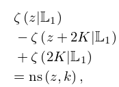
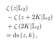
… ►In this subsection $2{\omega }_1$, $2{\omega }_3$ are any pair of generators of the lattice $𝕃$, and the lattice roots $e_1$, $e_2$, $e_3$ are given by (23.3.9). … ►Again, in Equations (23.6.16)–(23.6.26), $2{\omega }_1,2{\omega }_3$ are any pair of generators of the lattice $𝕃$ and $e_1,e_2,e_3$ are given by (23.3.9). … ►Also, ${𝕃}_1$, ${𝕃}_2$, ${𝕃}_3$ are the lattices with generators $(4K,2\mathrm{i}{K}^{\prime })$, $(2K-2\mathrm{i}{K}^{\prime },2K+2\mathrm{i}{K}^{\prime })$, $(2K,4\mathrm{i}{K}^{\prime })$, respectively. ►

23.6.27 $$\zeta \left(z|{𝕃}_1\right)-\zeta \left(z+2K|{𝕃}_1\right)+\zeta \left(2K|{𝕃}_1\right)=\mathrm{ns}(z,k),$$

ⓘ

Symbols:

$\mathrm{ns}(z,k)$: Jacobian elliptic function, $\zeta \left(z\right)$ (= $\zeta \left(z|𝕃\right)$ = $\zeta (z;g_2,g_3)$): Weierstrass zeta function, $K\left(k\right)$: Legendre’s complete elliptic integral of the first kind, $𝕃$: lattice, $z$: complex and $k$: modulus

Referenced by:

§23.6(ii), §23.6(ii)

Permalink:

http://dlmf.nist.gov/23.6.E27

Encodings:

pMML, png, TeX

See also:

Annotations for §23.6(ii), §23.6 and Ch.23

►

23.6.28 $$\zeta \left(z|{𝕃}_2\right)-\zeta \left(z+2K|{𝕃}_2\right)+\zeta \left(2K|{𝕃}_2\right)=\mathrm{ds}(z,k),$$

ⓘ

Symbols:

$\mathrm{ds}(z,k)$: Jacobian elliptic function, $\zeta \left(z\right)$ (= $\zeta \left(z|𝕃\right)$ = $\zeta (z;g_2,g_3)$): Weierstrass zeta function, $K\left(k\right)$: Legendre’s complete elliptic integral of the first kind, $𝕃$: lattice, $z$: complex and $k$: modulus

Permalink:

http://dlmf.nist.gov/23.6.E28

Encodings:

pMML, png, TeX

See also:

Annotations for §23.6(ii), §23.6 and Ch.23

…

28: 23.11 Integral Representations

… ►

23.11.2 $$\mathrm{\wp }\left(z\right)=\frac{1}{z^2}+8{\int }_0^{\mathrm{\infty }}s\left({\mathrm{e}}^{-s}{\sinh }^2\left(\frac{1}{2}zs\right)f_1(s,\tau )+{\mathrm{e}}^{\mathrm{i}\tau s}{\sin }^2\left(\frac{1}{2}zs\right)f_2(s,\tau )\right)ds,$$

ⓘ

Symbols:

$\mathrm{\wp }\left(z\right)$ (= $\mathrm{\wp }\left(z|𝕃\right)$ = $\mathrm{\wp }(z;g_2,g_3)$): Weierstrass $\mathrm{\wp }$-function, $dx$: differential of $x$ , $\mathrm{e}$: base of natural logarithm, $\sinh z$: hyperbolic sine function, $\mathrm{i}$: imaginary unit, $\int$: integral, $\sin z$: sine function, $𝕃$: lattice, $z$: complex, $\tau$: complex variable and $f_j(s,\tau )$: functions

Permalink:

http://dlmf.nist.gov/23.11.E2

Encodings:

pMML, png, TeX

See also:

Annotations for §23.11 and Ch.23

… ►

23.11.3 $$\zeta \left(z\right)=\frac{1}{z}+{\int }_0^{\mathrm{\infty }}\left({\mathrm{e}}^{-s}\left(zs-\sinh \left(zs\right)\right)f_1(s,\tau )-{\mathrm{e}}^{\mathrm{i}\tau s}\left(zs-\sin \left(zs\right)\right)f_2(s,\tau )\right)ds,$$

ⓘ

Symbols:

$\zeta \left(z\right)$ (= $\zeta \left(z|𝕃\right)$ = $\zeta (z;g_2,g_3)$): Weierstrass zeta function, $dx$: differential of $x$ , $\mathrm{e}$: base of natural logarithm, $\sinh z$: hyperbolic sine function, $\mathrm{i}$: imaginary unit, $\int$: integral, $\sin z$: sine function, $𝕃$: lattice, $z$: complex, $\tau$: complex variable and $f_j(s,\tau )$: functions

Permalink:

http://dlmf.nist.gov/23.11.E3

Encodings:

pMML, png, TeX

See also:

Annotations for §23.11 and Ch.23

…

29: 23.12 Asymptotic Approximations

… ►

23.12.1 $$\mathrm{\wp }\left(z\right)=\frac{{\pi }^2}{4{\omega }_1^2}\left(-\frac{1}{3}+{\csc }^2\left(\frac{\pi z}{2{\omega }_1}\right)+8\left(1-\cos \left(\frac{\pi z}{{\omega }_1}\right)\right)q^2+O\left(q^4\right)\right),$$

ⓘ

Symbols:

$O\left(x\right)$: order not exceeding, $\mathrm{\wp }\left(z\right)$ (= $\mathrm{\wp }\left(z|𝕃\right)$ = $\mathrm{\wp }(z;g_2,g_3)$): Weierstrass $\mathrm{\wp }$-function, $\pi$: the ratio of the circumference of a circle to its diameter, $\csc z$: cosecant function, $\cos z$: cosine function, $𝕃$: lattice, $q$: nome, $z$: complex and ${\omega }_1$, ${\omega }_3$, ${\omega }_2=-{\omega }_1-{\omega }_3$: lattice generators

Referenced by:

§23.12

Permalink:

http://dlmf.nist.gov/23.12.E1

Encodings:

pMML, png, TeX

See also:

Annotations for §23.12 and Ch.23

►

23.12.2 $$\zeta \left(z\right)=\frac{{\pi }^2}{4{\omega }_1^2}\left(\frac{z}{3}+\frac{2{\omega }_1}{\pi }\cot \left(\frac{\pi z}{2{\omega }_1}\right)-8\left(z-\frac{{\omega }_1}{\pi }\sin \left(\frac{\pi z}{{\omega }_1}\right)\right)q^2+O\left(q^4\right)\right),$$

ⓘ

Symbols:

$O\left(x\right)$: order not exceeding, $\zeta \left(z\right)$ (= $\zeta \left(z|𝕃\right)$ = $\zeta (z;g_2,g_3)$): Weierstrass zeta function, $\pi$: the ratio of the circumference of a circle to its diameter, $\cot z$: cotangent function, $\sin z$: sine function, $𝕃$: lattice, $q$: nome, $z$: complex and ${\omega }_1$, ${\omega }_3$, ${\omega }_2=-{\omega }_1-{\omega }_3$: lattice generators

Referenced by:

§23.12, Erratum (V1.0.23) for Equation (23.12.2)

Permalink:

http://dlmf.nist.gov/23.12.E2

Encodings:

pMML, png, TeX

Correction (effective with 1.0.23):

The factor of 2, previously omitted from the denominator of the argument of the $\cot$ function has been inserted.

Suggested 2019-05-27 by Blagoje Oblak

See also:

Annotations for §23.12 and Ch.23

►

23.12.3 $$\sigma \left(z\right)=\frac{2{\omega }_1}{\pi }\exp \left(\frac{{\pi }^2{z}^2}{24{\omega }_1^2}\right)\sin \left(\frac{\pi z}{2{\omega }_1}\right)\left(1-\left(\frac{{\pi }^2{z}^2}{{\omega }_1^2}-4{\sin }^2\left(\frac{\pi z}{2{\omega }_1}\right)\right)q^2+O\left(q^4\right)\right),$$

ⓘ

Symbols:

$O\left(x\right)$: order not exceeding, $\sigma \left(z\right)$ (= $\sigma \left(z|𝕃\right)$ = $\sigma (z;g_2,g_3)$): Weierstrass sigma function, $\pi$: the ratio of the circumference of a circle to its diameter, $\exp z$: exponential function, $\sin z$: sine function, $𝕃$: lattice, $q$: nome, $z$: complex and ${\omega }_1$, ${\omega }_3$, ${\omega }_2=-{\omega }_1-{\omega }_3$: lattice generators

Permalink:

http://dlmf.nist.gov/23.12.E3

Encodings:

pMML, png, TeX

See also:

Annotations for §23.12 and Ch.23

►provided that $z\notin 𝕃$ in the case of (23.12.1) and (23.12.2). …

30: 18.6 Symmetry, Special Values, and Limits to Monomials

… ►

18.6.1 $$L_n^{(\alpha )}\left(0\right)=\frac{{\left(\alpha +1\right)}_n}{n!}.$$

ⓘ

Symbols:

$L_n^{(\alpha )}\left(x\right)$: Laguerre (or generalized Laguerre) polynomial, ${\left(a\right)}_n$: Pochhammer’s symbol (or shifted factorial), $!$: factorial (as in $n!$) and $n$: nonnegative integer

A&S Ref:

22.4.7 (see column for $f_n(0)$)

Referenced by:

§18.17(i), §18.6(i), §18.6(ii)

Permalink:

http://dlmf.nist.gov/18.6.E1

Encodings:

pMML, png, TeX

See also:

Annotations for §18.6(i), §18.6(i), §18.6 and Ch.18

… ►

18.6.5 $$\underset{\alpha \to \mathrm{\infty }}{lim}\frac{L_n^{(\alpha )}\left(\alpha x\right)}{L_n^{(\alpha )}\left(0\right)}={(1-x)}^n.$$

ⓘ

Symbols:

$L_n^{(\alpha )}\left(x\right)$: Laguerre (or generalized Laguerre) polynomial, $n$: nonnegative integer and $x$: real variable

Referenced by:

§18.6(ii)

Permalink:

http://dlmf.nist.gov/18.6.E5

Encodings:

pMML, png, TeX

See also:

Annotations for §18.6(ii), §18.6 and Ch.18