L%E2%80%99H%C3%B4pital%20rule
(0.002 seconds)
21—30 of 325 matching pages
21: 23.19 Interrelations
…
►
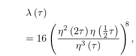
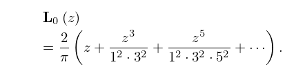
23.19.1
…
►
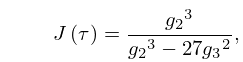
23.19.3
►where are the invariants of the lattice with generators and ; see §23.3(i).
…
►
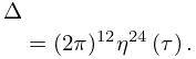
23.19.4
22: 11.7 Integrals and Sums
…
►
…
►For integrals of and with respect to the order , see Apelblat (1989).
…
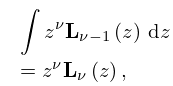
11.7.3
►
11.7.4
…
►The following Laplace transforms of require for convergence, while those of require .
…
►
23: 11.13 Methods of Computation
…
►For a review of methods for the computation of see Zanovello (1975).
For simple and effective approximations to and see Aarts and Janssen (2016).
…
►Subsequently and are obtainable via (11.2.5) and (11.2.6).
…
►Then from the limiting forms for small argument (§§11.2(i), 10.7(i), 10.30(i)), limiting forms for large argument (§§11.6(i), 10.7(ii), 10.30(ii)), and the connection formulas (11.2.5) and (11.2.6), it is seen that and can be computed in a stable manner by integrating forwards, that is, from the origin toward infinity.
…
►Sequences of values of and , with fixed, can be computed by application of the inhomogeneous difference equations (11.4.23) and (11.4.25).
…
24: Bibliography
…
►
Algorithm 683: A portable FORTRAN subroutine for exponential integrals of a complex argument.
ACM Trans. Math. Software 16 (2), pp. 178–182.
…
►
Applications of basic hypergeometric functions.
SIAM Rev. 16 (4), pp. 441–484.
…
►
Derivatives and integrals with respect to the order of the Struve functions and
.
J. Math. Anal. Appl. 137 (1), pp. 17–36.
…
►
Note on the trivial zeros of Dirichlet -functions.
Proc. Amer. Math. Soc. 94 (1), pp. 29–30.
…
►
Quadratic differentials and asymptotics of Laguerre polynomials with varying complex parameters.
J. Math. Anal. Appl. 416 (1), pp. 52–80.
…
25: 19.9 Inequalities
…
►The perimeter of an ellipse with semiaxes is given by
…Almkvist and Berndt (1988) list thirteen approximations to that have been proposed by various authors.
…Ramanujan’s approximation and its leading error term yield the following approximation to :
…Even for the extremely eccentric ellipse with and , this is correct within 0.
…
►where
…
26: 11.2 Definitions
…
►
11.2.2
…
►The functions and are entire functions of and .
…
►
11.2.4
…
►Unless indicated otherwise, , , , and assume their principal values throughout the DLMF.
…
►
11.2.10
…
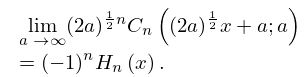
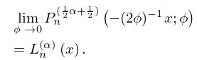
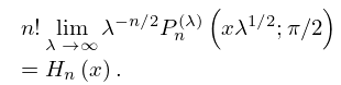
27: 18.7 Interrelations and Limit Relations
28: 18.21 Hahn Class: Interrelations
29: 3.2 Linear Algebra
…
►With the process of solution can then be regarded as first solving the equation for (forward
elimination), followed by the solution of for (back substitution).
…
►Because of rounding errors, the residual vector
is nonzero as a rule.
…
►(We are assuming that the matrix is real; if not is replaced by , the transpose of the complex conjugate of .)
…
►In the case that the orthogonality condition is replaced by -orthogonality, that is, , , for some positive definite matrix with Cholesky decomposition , then the details change as follows.
…
►
…
