Hurwitz criterion for stable polynomials

SearchAdvancedHelp

(0.002 seconds)

11—20 of 277 matching pages

11: Bibliography B

… ►

The generating function of Jacobi polynomials. J. London Math. Soc. 13, pp. 8–12.

ⓘ

External Links:

ISSN 0024-6107; 1469-7750/e, Document, ZentralBlatt

Referenced by:

§18.18(vii).

Encodings:

BibTeX

… ►

A generalisation of the Legendre polynomial. Proc. London Math. Soc. (2) 3 (3), pp. 111–123.

ⓘ

Notes:

Reviewed in JFM 36.0512.01

External Links:

Document, ZentralBlatt

Referenced by:

§18.12.

Encodings:

BibTeX

… ►

Polynomials defined by a difference system. J. Math. Anal. Appl. 2 (2), pp. 223–263.

ⓘ

External Links:

Document, MathReview (F. L. Spitzer), ZentralBlatt

Referenced by:

§18.33(v).

Encodings:

BibTeX

… ►

On the Hurwitz zeta-function. Rocky Mountain J. Math. 2 (1), pp. 151–157.

ⓘ

External Links:

MathReview (K. Thanigasalam), ZentralBlatt

Referenced by:

(25.11.26).

Encodings:

BibTeX

… ►

Criterion for Existence of a Bound State In One Dimension. American Journal of Physics 68 (2), pp. 160–161.

ⓘ

External Links:

Document

Referenced by:

§1.18(viii).

Encodings:

BibTeX

…

12: 8.15 Sums

… ►

8.15.2 $$a\sum _{k=1}^{\mathrm{\infty }}\left(\frac{{\mathrm{e}}^{2\pi \mathrm{i}k(z+h)}}{{\left(2\pi \mathrm{i}k\right)}^{a+1}}\mathrm{\Gamma }(a,2\pi \mathrm{i}kz)+\frac{{\mathrm{e}}^{-2\pi \mathrm{i}k(z+h)}}{{\left(-2\pi \mathrm{i}k\right)}^{a+1}}\mathrm{\Gamma }(a,-2\pi \mathrm{i}kz)\right)=\zeta (-a,z+h)+\frac{z^{a+1}}{a+1}+\left(h-\frac{1}{2}\right)z^a,$$ $h\in [0,1]$.

ⓘ

Symbols:

$\zeta (s,a)$: Hurwitz zeta function, $\pi$: the ratio of the circumference of a circle to its diameter, $[a,b]$: closed interval, $\in$: element of, $\mathrm{e}$: base of natural logarithm, $\mathrm{i}$: imaginary unit, $\mathrm{\Gamma }(a,z)$: incomplete gamma function, $z$: complex variable, $a$: parameter and $k$: nonnegative integer

Proof sketch:

Start with and $z>0$. For $\mathrm{\Gamma }(a,\pm 2\pi \mathrm{i}kz)$ take integral representation (8.2.2) and use the substitution $t=\pm 2\pi \mathrm{i}kz(1+\tau )$. The sum and the integral can be interchanged, and the sum can be evaluated via (4.6.1). Use integration by parts. This will result in $\left(h-\frac{1}{2}\right)z^a$ plus two integrals with infinitely many poles. The residue theorem (§1.10(iv)) will give us an infinite series which can be identified via (25.11.1). For other values of $a$ and $z$ use analytic continuation.

Referenced by:

§25.11(x), §25.11(x), §8.15, Erratum (V1.1.3) for Additions

Permalink:

http://dlmf.nist.gov/8.15.E2

Encodings:

pMML, png, TeX

Addition (effective with 1.1.3):

This equation was added.

See also:

Annotations for §8.15 and Ch.8

►For the Hurwitz zeta function $\zeta (s,a)$ see §25.11(i). …

13: 25.19 Tables

… ►

Cloutman (1989) tabulates $\mathrm{\Gamma }\left(s+1\right)F_s(x)$, where $F_s(x)$ is the Fermi–Dirac integral (25.12.14), for $s=-\frac{1}{2},\frac{1}{2},\frac{3}{2},\frac{5}{2}$, $x=-5(.05)25$, to 12S.

►

Fletcher et al. (1962, §22.1) lists many sources for earlier tables of $\zeta \left(s\right)$ for both real and complex $s$. §22.133 gives sources for numerical values of coefficients in the Riemann–Siegel formula, §22.15 describes tables of values of $\zeta (s,a)$, and §22.17 lists tables for some Dirichlet $L$-functions for real characters. For tables of dilogarithms, polylogarithms, and Clausen’s integral see §§22.84–22.858.

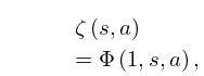
14: 25.14 Lerch’s Transcendent

… ►The Hurwitz zeta function $\zeta (s,a)$ (§25.11) and the polylogarithm ${\mathrm{Li}}_s\left(z\right)$ (§25.12(ii)) are special cases: ►

25.14.2 $$\zeta (s,a)=\mathrm{\Phi }(1,s,a),$$ $\mathrm{\Re }s>1$, $a\ne 0,-1,-2,\mathrm{\dots }$,

ⓘ

Symbols:

$\zeta (s,a)$: Hurwitz zeta function, $\mathrm{\Phi }(z,s,a)$: Lerch’s transcendent, $\mathrm{\Re }$: real part, $a$: real or complex parameter and $s$: complex variable

Keywords:

specialization

Proof sketch:

Derivable from (25.11.1), (25.14.1).

Permalink:

http://dlmf.nist.gov/25.14.E2

Encodings:

pMML, png, TeX

See also:

Annotations for §25.14(i), §25.14 and Ch.25

…

15: 25.21 Software

… ►

§25.21(iv) Hurwitz Zeta Function

…

16: 24.16 Generalizations

§24.16 Generalizations

… ►

Polynomials and Numbers of Integer Order

… ►

Nörlund Polynomials

… ►

§24.16(ii) Character Analogs

… ►In no particular order, other generalizations include: Bernoulli numbers and polynomials with arbitrary complex index (Butzer et al. (1992)); Euler numbers and polynomials with arbitrary complex index (Butzer et al. (1994)); q-analogs (Carlitz (1954a), Andrews and Foata (1980)); conjugate Bernoulli and Euler polynomials (Hauss (1997, 1998)); Bernoulli–Hurwitz numbers (Katz (1975)); poly-Bernoulli numbers (Kaneko (1997)); Universal Bernoulli numbers (Clarke (1989)); $p$-adic integer order Bernoulli numbers (Adelberg (1996)); $p$-adic $q$-Bernoulli numbers (Kim and Kim (1999)); periodic Bernoulli numbers (Berndt (1975b)); cotangent numbers (Girstmair (1990b)); Bernoulli–Carlitz numbers (Goss (1978)); Bernoulli–Padé numbers (Dilcher (2002)); Bernoulli numbers belonging to periodic functions (Urbanowicz (1988)); cyclotomic Bernoulli numbers (Girstmair (1990a)); modified Bernoulli numbers (Zagier (1998)); higher-order Bernoulli and Euler polynomials with multiple parameters (Erdélyi et al. (1953a, §§1.13.1, 1.14.1)).

17: Bibliography N

… ►

Error bounds for the asymptotic expansion of the Hurwitz zeta function. Proc. A. 473 (2203), pp. 20170363, 16.

ⓘ

External Links:

ISSN 1364-5021, Document, Link, MathReview Entry, ZentralBlatt

Referenced by:

§8.15.

Encodings:

BibTeX

… ►

Orthogonal polynomials. Mem. Amer. Math. Soc. 18 (213), pp. v+185 pp..

ⓘ

External Links:

ISSN 0065-9266, Document, Link, MathReview (T. S. Chihara)

Referenced by:

§18.2(xi), §18.2(xi).

Encodings:

BibTeX

►

Géza Freud, orthogonal polynomials and Christoffel functions. A case study. J. Approx. Theory 48 (1), pp. 3–167.

ⓘ

External Links:

ISSN 0021-9045, Document, MathReview (T. S. Chihara), ZentralBlatt

Referenced by:

§18.32.

Encodings:

BibTeX

… ►

Askey-Wilson polynomials: an affine Hecke algebra approach. In Laredo Lectures on Orthogonal Polynomials and Special Functions, Adv. Theory Spec. Funct. Orthogonal Polynomials, pp. 111–144.

ⓘ

External Links:

MathReview (V. L. Deshpande), ZentralBlatt

Referenced by:

§18.38(iii).

Encodings:

BibTeX

… ►

Symmetries in the fourth Painlevé equation and Okamoto polynomials. Nagoya Math. J. 153, pp. 53–86.

ⓘ

External Links:

ISSN 0027-7630, MathReview (Andrei A. Kapaev), ZentralBlatt

Referenced by:

§32.8(iv).

Encodings:

BibTeX

…

18: Bibliography P

… ►

The Stokes phenomenon associated with the Hurwitz zeta function $\zeta (s,a)$ . Proc. Roy. Soc. London Ser. A 461, pp. 297–304.

ⓘ

External Links:

ISSN 1364-5021, Document, MathReview (Marc Prevost), ZentralBlatt

Referenced by:

(25.11.43), §25.11(xii).

Encodings:

BibTeX

… ►

Zonal Polynomials of Order $1$ Through $12$ . In Selected Tables in Mathematical Statistics, H. L. Harter and D. B. Owen (Eds.), Vol. 2, pp. 199–388.

ⓘ

External Links:

MathReview

Referenced by:

§35.11.

Encodings:

BibTeX

… ►

Orthogonal polynomials and some $q$-beta integrals of Ramanujan. J. Math. Anal. Appl. 112 (2), pp. 517–540.

ⓘ

External Links:

ISSN 0022-247X, Document, MathReview (Mourad E. H. Ismail), ZentralBlatt

Referenced by:

§18.33(iv), §18.33(v).

Encodings:

BibTeX

… ►

A new basis for the representation of the rotation group. Lamé and Heun polynomials. J. Mathematical Phys. 14 (8), pp. 1130–1139.

ⓘ

External Links:

Document, ZentralBlatt

Referenced by:

§29.18(iv).

Encodings:

BibTeX

… ►

Chebyshev polynomial expansions of the Riemann zeta function. Math. Comp. 26 (120), pp. G1–G5.

ⓘ

External Links:

ISSN 0025-5718, FullText, MathReview

Referenced by:

2nd item, 3rd item.

Encodings:

BibTeX

…

19: Bibliography R

… ►

A non-negative representation of the linearization coefficients of the product of Jacobi polynomials. Canad. J. Math. 33 (4), pp. 915–928.

ⓘ

External Links:

ISSN 0008-414X, Document, Link, MathReview (R. A. Askey), ZentralBlatt

Referenced by:

§18.18(v).

Encodings:

BibTeX

►

The Associated Classical Orthogonal Polynomials. In Special Functions 2000: Current Perspective and Future Directions (Tempe, AZ), NATO Sci. Ser. II Math. Phys. Chem., Vol. 30, pp. 255–279.

ⓘ

External Links:

MathReview (Wadim Zudilin), ZentralBlatt

Referenced by:

§18.30(viii).

Encodings:

BibTeX

… ►

Relationships between the zeros, weights, and weight functions of orthogonal polynomials: Derivative rule approach to Stieltjes and spectral imaging. Computing in Science and Engineering 23 (3), pp. 56–64.

ⓘ

External Links:

ISSN 1521-9615, Document, Link

Referenced by:

§18.39(iv), §18.40(ii).

Encodings:

BibTeX

… ►

Infinite Sum of the Incomplete Gamma Function Expressed in Terms of the Hurwitz Zeta Function. Mathematics 9 (16).

ⓘ

External Links:

Link, ISSN 2227-7390, Document

Referenced by:

§8.15.

Encodings:

BibTeX

… ►

Hypergeometric Functions on Domains of Positivity, Jack Polynomials, and Applications. Contemporary Mathematics, Vol. 138, American Mathematical Society, Providence, RI.

ⓘ

External Links:

ISBN 0-8218-5159-4, MathReview, ZentralBlatt

Referenced by:

Ch.35, Profile Donald St. P. Richards.

Encodings:

BibTeX

…

20: 28.17 Stability as $x\to \pm \mathrm{\infty }$

§28.17 Stability as $x\to \pm \mathrm{\infty }$

►If all solutions of (28.2.1) are bounded when $x\to \pm \mathrm{\infty }$ along the real axis, then the corresponding pair of parameters $(a,q)$ is called stable. … ►For example, positive real values of $a$ with $q=0$ comprise stable pairs, as do values of $a$ and $q$ that correspond to real, but noninteger, values of $\nu$. … ►For real $a$ and $q$ $(\ne 0)$ the stable regions are the open regions indicated in color in Figure 28.17.1. … ►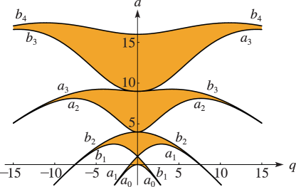

►►

Figure 28.17.1: Stability chart for eigenvalues of Mathieu’s equation (28.2.1). Magnify