Heine%20integral
(0.002 seconds)
21—30 of 475 matching pages
21: 7.24 Approximations
§7.24(i) Approximations in Terms of Elementary Functions
… ►Cody (1969) provides minimax rational approximations for and . The maximum relative precision is about 20S.
Cody et al. (1970) gives minimax rational approximations to Dawson’s integral (maximum relative precision 20S–22S).
Luke (1969b, vol. 2, pp. 422–435) gives main diagonal Padé approximations for , , , , and ; approximate errors are given for a selection of -values.
22: 25.12 Polylogarithms
Integral Representation
… ►§25.12(iii) Fermi–Dirac and Bose–Einstein Integrals
►The Fermi–Dirac and Bose–Einstein integrals are defined by … ►In terms of polylogarithms …23: 22.3 Graphics
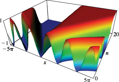
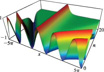
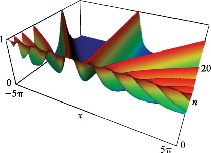
 ►
►
24: 10.75 Tables
Achenbach (1986) tabulates , , , , , 20D or 18–20S.
Zhang and Jin (1996, p. 270) tabulates , , , , , 8D.
Bickley et al. (1952) tabulates or , or , , (.01 or .1) 10(.1) 20, 8S; , , , or , 10S.
Kerimov and Skorokhodov (1984b) tabulates all zeros of the principal values of and , for , 9S.
Zhang and Jin (1996, p. 271) tabulates , , , , , 8D.
25: 6.16 Mathematical Applications
§6.16(i) The Gibbs Phenomenon
… ►Hence, if is fixed and , then , , or according as , , or ; compare (6.2.14). … ►The first maximum of for positive occurs at and equals ; compare Figure 6.3.2. … ►§6.16(ii) Number-Theoretic Significance of
►If we assume Riemann’s hypothesis that all nonreal zeros of have real part of (§25.10(i)), then …26: 25.20 Approximations
Cody et al. (1971) gives rational approximations for in the form of quotients of polynomials or quotients of Chebyshev series. The ranges covered are , , , . Precision is varied, with a maximum of 20S.
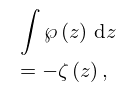
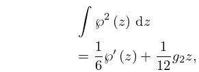
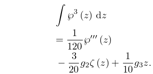
27: 23.14 Integrals
§23.14 Integrals
►28: 9.18 Tables
Zhang and Jin (1996, p. 337) tabulates , , , for to 8S and for to 9D.
Sherry (1959) tabulates , , , , ; 20S.
Zhang and Jin (1996, p. 339) tabulates , , , , , , , , ; 8D.
§9.18(v) Integrals
…29: 7.23 Tables
Abramowitz and Stegun (1964, Chapter 7) includes , , , 10D; , , 8S; , , 7D; , , , 6S; , , 10D; , , 9D; , , , 7D; , , , , 15D.
Abramowitz and Stegun (1964, Table 27.6) includes the Goodwin–Staton integral , , 4D; also , , 4D.
Zhang and Jin (1996, pp. 637, 639) includes , , , 8D; , , , 8D.
Zhang and Jin (1996, pp. 638, 640–641) includes the real and imaginary parts of , , , 7D and 8D, respectively; the real and imaginary parts of , , , 8D, together with the corresponding modulus and phase to 8D and 6D (degrees), respectively.
Zhang and Jin (1996, p. 642) includes the first 10 zeros of , 9D; the first 25 distinct zeros of and , 8S.
