Euler pentagonal number theorem
(0.002 seconds)
31—40 of 539 matching pages
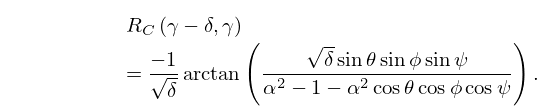
31: 19.11 Addition Theorems
32: 25.15 Dirichlet -functions
…
►For the principal character , is analytic everywhere except for a simple pole at with residue , where is Euler’s totient function (§27.2).
…
►
25.15.5
…
►This result plays an important role in the proof of Dirichlet’s theorem on primes in arithmetic progressions (§27.11).
Related results are:
►
25.15.10
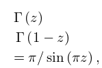
33: 5.5 Functional Relations
…
►
5.5.1
…
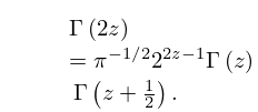
►
5.5.3
,
…
►
5.5.5
…
►
§5.5(iv) Bohr–Mollerup Theorem
►If a positive function on satisfies , , and is convex (see §1.4(viii)), then .34: 31.14 General Fuchsian Equation
…
►The general second-order Fuchsian equation with regular singularities at , , and at , is given by
…The exponents at the finite singularities are and those at are , where
…The three sets of parameters comprise the singularity parameters
, the exponent parameters
, and the free accessory parameters
.
With and the total number of free parameters is .
…
►
31.14.3
…
35: 27.21 Tables
§27.21 Tables
… ►Glaisher (1940) contains four tables: Table I tabulates, for all : (a) the canonical factorization of into powers of primes; (b) the Euler totient ; (c) the divisor function ; (d) the sum of these divisors. Table II lists all solutions of the equation for all , where is defined by (27.14.2). …6 lists , and for ; Table 24. … ►36: 25.2 Definition and Expansions
…
►where the Stieltjes constants are defined via
…
►
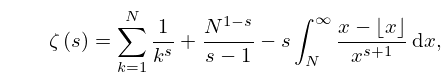
§25.2(iii) Representations by the Euler–Maclaurin Formula
►
25.2.8
, .
…
►For see §24.2(i), and for see §24.2(iii).
…
►product over zeros of with (see §25.10(i)); is Euler’s constant (§5.2(ii)).
37: 25.1 Special Notation
…
►
►
…
| nonnegative integers. | |
| prime number. | |
| … | |
| Euler’s constant (§5.2(ii)). | |
| digamma function except in §25.16. See §5.2(i). | |
| Bernoulli number and polynomial (§24.2(i)). | |
| … | |
38: 5.18 -Gamma and -Beta Functions
…
►
5.18.5
…
►
5.18.7
►Also, is convex for , and the analog of the Bohr–Mollerup theorem (§5.5(iv)) holds.
…
►For generalized asymptotic expansions of as see Olde Daalhuis (1994) and Moak (1984).
For the -digamma or -psi function see Salem (2013).
…
39: Karl Dilcher
…
►Dilcher’s research interests include classical analysis, special functions, and elementary, combinatorial, and computational number theory.
Over the years he authored or coauthored numerous papers on Bernoulli numbers and related topics, and he maintains a large on-line bibliography on the subject.
…
►
…
40: 25.10 Zeros
…
►Also, for , a property first established in Hadamard (1896) and de la Vallée Poussin (1896a, b) in the proof of the prime number theorem (25.16.3).
…
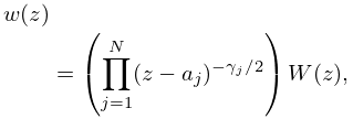
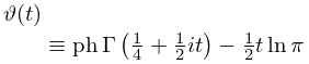
►
25.10.2
►is chosen to make real, and assumes its principal value.
…
►Riemann developed a method for counting the total number
of zeros of in that portion of the critical strip with .
By comparing with the number of sign changes of we can decide whether has any zeros off the line in this region.
…
