Euler–Poisson–Darboux equation
(0.002 seconds)
21—30 of 622 matching pages
21: 18.12 Generating Functions
…
►
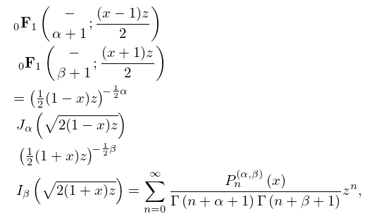
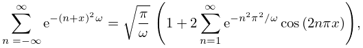
18.12.2
►
18.12.2_5
, ,
►with arbitrary.
Note that (18.12.2_5) yields (18.12.1) by putting and (18.12.2) by replacing by and next letting .
…
►See §18.18(vii) for Poisson kernels; these are special cases of bilateral generating functions.
22: 24.4 Basic Properties
…
►
§24.4(i) Difference Equations
… ►§24.4(ii) Symmetry
… ►§24.4(iii) Sums of Powers
… ►§24.4(iv) Finite Expansions
… ►Next, …23: 31.14 General Fuchsian Equation
§31.14 General Fuchsian Equation
►§31.14(i) Definitions
… ►The exponents at the finite singularities are and those at are , where …The three sets of parameters comprise the singularity parameters , the exponent parameters , and the free accessory parameters . … ►Normal Form
…24: 30.6 Functions of Complex Argument
…
►The solutions
…of (30.2.1) with and are real when , and their principal values (§4.2(i)) are obtained by analytic continuation to .
…
►with as in (30.11.4).
…
►For results for Equation (30.2.1) with complex parameters see Meixner and Schäfke (1954).
25: 1.8 Fourier Series
…
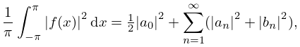
►
1.8.5
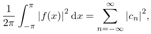
►
1.8.6
…
►
§1.8(iv) Poisson’s Summation Formula
►
1.8.13Moved to (1.8.6_1).
…
►
1.8.16
.
…
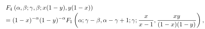
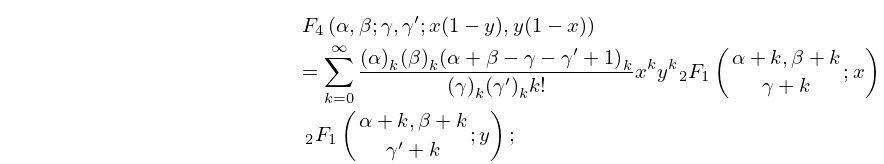
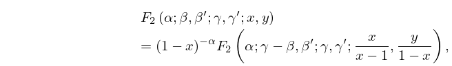
26: 16.16 Transformations of Variables
27: Bibliography W
…
►
Prime Divisors of the Bernoulli and Euler Numbers.
In Number Theory for the Millennium, III (Urbana, IL, 2000),
pp. 357–374.
…
►
The zeros of Euler’s psi function and its derivatives.
J. Math. Anal. Appl. 332 (1), pp. 607–616.
…
►
Linear difference equations with transition points.
Math. Comp. 74 (250), pp. 629–653.
…
►
The method of Darboux.
J. Approximation Theory 10 (2), pp. 159–171.
…
►
On a uniform treatment of Darboux’s method.
Constr. Approx. 21 (2), pp. 225–255.
…
28: 15.11 Riemann’s Differential Equation
§15.11 Riemann’s Differential Equation
… ►The most general form is given by … ►Here , , are the exponent pairs at the points , , , respectively. …Also, if any of , , , is at infinity, then we take the corresponding limit in (15.11.1). … ►These constants can be chosen to map any two sets of three distinct points and onto each other. …29: 20.11 Generalizations and Analogs
…
►This is the discrete analog of the Poisson identity (§1.8(iv)).
…
►The first of equations (20.9.2) can also be written
…
►The importance of these combined theta functions is that sets of twelve equations for the theta functions often can be replaced by corresponding sets of three equations of the combined theta functions, plus permutation symmetry.
Such sets of twelve equations include derivatives, differential equations, bisection relations, duplication relations, addition formulas (including new ones for theta functions), and pseudo-addition formulas.
…
