3j symbols

(0.013 seconds)

11—20 of 91 matching pages

11: 34.9 Graphical Method

§34.9 Graphical Method

… ►For specific examples of the graphical method of representing sums involving the

\mathit{3j},\mathit{6j}

, and

\mathit{9j}

symbols, see Varshalovich et al. (1988, Chapters 11, 12) and Lehman and O’Connell (1973, §3.3).

12: 34.6 Definition: $\mathit{9j}$ Symbol

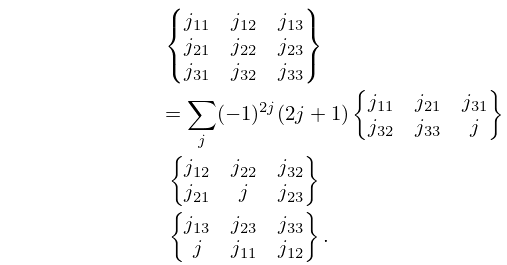
… ►The

\mathit{9j}

symbol may be defined either in terms of

\mathit{3j}

symbols or equivalently in terms of

\mathit{6j}

symbols: ►

34.6.1

\begin{Bmatrix}j_{11}&j_{12}&j_{13}\\ j_{21}&j_{22}&j_{23}\\ j_{31}&j_{32}&j_{33}\end{Bmatrix}=\sum_{\mbox{\scriptsize all }m_{rs}}\begin{% pmatrix}j_{11}&j_{12}&j_{13}\\ m_{11}&m_{12}&m_{13}\end{pmatrix}\begin{pmatrix}j_{21}&j_{22}&j_{23}\\ m_{21}&m_{22}&m_{23}\end{pmatrix}\begin{pmatrix}j_{31}&j_{32}&j_{33}\\ m_{31}&m_{32}&m_{33}\end{pmatrix}\*\begin{pmatrix}j_{11}&j_{21}&j_{31}\\ m_{11}&m_{21}&m_{31}\end{pmatrix}\begin{pmatrix}j_{12}&j_{22}&j_{32}\\ m_{12}&m_{22}&m_{32}\end{pmatrix}\begin{pmatrix}j_{13}&j_{23}&j_{33}\\ m_{13}&m_{23}&m_{33}\end{pmatrix},

ⓘ

Defines:: $\begin{Bmatrix}\NVar{j_{11}}&\NVar{j_{12}}&\NVar{j_{13}}\\ \NVar{j_{21}}&\NVar{j_{22}}&\NVar{j_{23}}\\ \NVar{j_{31}}&\NVar{j_{32}}&\NVar{j_{33}}\end{Bmatrix}$ : $\mathit{9j}$ symbol
Symbols:: $\begin{pmatrix}\NVar{j_{1}}&\NVar{j_{2}}&\NVar{j_{3}}\\ \NVar{m_{1}}&\NVar{m_{2}}&\NVar{m_{3}}\end{pmatrix}$ : $\mathit{3j}$ symbol, $j,j_{r}$ : non-negative integers or non-negative integers plus one half., $r$ : nonnegative integer and $s$ : integer
Permalink:: http://dlmf.nist.gov/34.6.E1
Encodings:: pMML, png, TeX
See also:: Annotations for §34.6 and Ch.34

►

34.6.2

\begin{Bmatrix}j_{11}&j_{12}&j_{13}\\ j_{21}&j_{22}&j_{23}\\ j_{31}&j_{32}&j_{33}\end{Bmatrix}=\sum_{j}(-1)^{2j}(2j+1)\begin{Bmatrix}j_{11}% &j_{21}&j_{31}\\ j_{32}&j_{33}&j\end{Bmatrix}\begin{Bmatrix}j_{12}&j_{22}&j_{32}\\ j_{21}&j&j_{23}\end{Bmatrix}\begin{Bmatrix}j_{13}&j_{23}&j_{33}\\ j&j_{11}&j_{12}\end{Bmatrix}.

ⓘ

Symbols:: $\begin{Bmatrix}\NVar{j_{11}}&\NVar{j_{12}}&\NVar{j_{13}}\\ \NVar{j_{21}}&\NVar{j_{22}}&\NVar{j_{23}}\\ \NVar{j_{31}}&\NVar{j_{32}}&\NVar{j_{33}}\end{Bmatrix}$ : $\mathit{9j}$ symbol, $\begin{Bmatrix}\NVar{j_{1}}&\NVar{j_{2}}&\NVar{j_{3}}\\ \NVar{l_{1}}&\NVar{l_{2}}&\NVar{l_{3}}\end{Bmatrix}$ : $\mathit{6j}$ symbol and $j,j_{r}$ : non-negative integers or non-negative integers plus one half.
Referenced by:: §34.13
Permalink:: http://dlmf.nist.gov/34.6.E2
Encodings:: pMML, png, TeX
See also:: Annotations for §34.6 and Ch.34

…

13: 18.38 Mathematical Applications

… ►

$3j$ and $6j$ Symbols

►The

3j

symbol (34.2.6), with an alternative expression as a terminating

{{}_{3}F_{2}}

of unit argument, can be expressed in terms of Hahn polynomials (18.20.5) or, by (18.21.1), dual Hahn polynomials. The orthogonality relations in §34.3(iv) for the

3j

symbols can be rewritten in terms of orthogonality relations for Hahn or dual Hahn polynomials as given by §§18.2(i), 18.2(iii) and Table 18.19.1 or by §18.25(iii), respectively. … ►The

6j

symbol (34.4.3), with an alternative expression as a terminating balanced

{{}_{4}F_{3}}

of unit argument, can be expressend in terms of Racah polynomials (18.26.3). …

14: 34.8 Approximations for Large Parameters

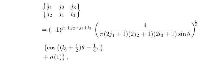
§34.8 Approximations for Large Parameters

►For large values of the parameters in the

\mathit{3j}

\mathit{6j}

, and

\mathit{9j}

symbols, different asymptotic forms are obtained depending on which parameters are large. … ►

34.8.1

\begin{Bmatrix}j_{1}&j_{2}&j_{3}\\ j_{2}&j_{1}&l_{3}\end{Bmatrix}=(-1)^{j_{1}+j_{2}+j_{3}+l_{3}}\*\left(\frac{4}{% \pi(2j_{1}+1)(2j_{2}+1)(2l_{3}+1)\sin\theta}\right)^{\frac{1}{2}}\*\left(\cos% \left((l_{3}+\tfrac{1}{2})\theta-\tfrac{1}{4}\pi\right)+o\left(1\right)\right),

j_{1},j_{2},j_{3}\gg l_{3}\gg 1

ⓘ

Symbols:: $\pi$ : the ratio of the circumference of a circle to its diameter, $\cos\NVar{z}$ : cosine function, $o\left(\NVar{x}\right)$ : order less than, $\sin\NVar{z}$ : sine function, $\begin{Bmatrix}\NVar{j_{1}}&\NVar{j_{2}}&\NVar{j_{3}}\\ \NVar{l_{1}}&\NVar{l_{2}}&\NVar{l_{3}}\end{Bmatrix}$ : $\mathit{6j}$ symbol, $j,j_{r}$ : non-negative integers or non-negative integers plus one half. and $l,l_{r}$ : non-negative integers or non-negative integers plus one half.
Permalink:: http://dlmf.nist.gov/34.8.E1
Encodings:: pMML, png, TeX
See also:: Annotations for §34.8 and Ch.34

… ►Uniform approximations in terms of Airy functions for the

\mathit{3j}

and

\mathit{6j}

symbols are given in Schulten and Gordon (1975b). For approximations for the

\mathit{3j}

\mathit{6j}

, and

\mathit{9j}

symbols with error bounds see Flude (1998), Chen et al. (1999), and Watson (1999): these references also cite earlier work.

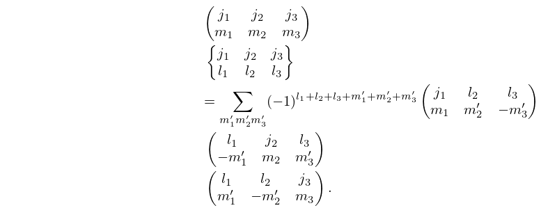
15: 34.4 Definition: $\mathit{6j}$ Symbol

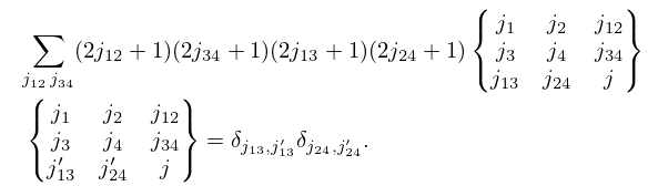
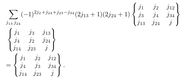
§34.4 Definition: $\mathit{6j}$ Symbol

►The

\mathit{6j}

symbol is defined by the following double sum of products of

\mathit{3j}

symbols: …where the summation is taken over all admissible values of the

m

’s and

m^{\prime}

’s for each of the four

\mathit{3j}

symbols; compare (34.2.2) and (34.2.3). ►Except in degenerate cases the combination of the triangle inequalities for the four

\mathit{3j}

symbols in (34.4.1) is equivalent to the existence of a tetrahedron (possibly degenerate) with edges of lengths

j_{1},j_{2},j_{3},l_{1},l_{2},l_{3}

; see Figure 34.4.1. … ►where

{{}_{4}F_{3}}

is defined as in §16.2. …

16: 16.4 Argument Unity

… ►See Raynal (1979) for a statement in terms of

\mathit{3j}

symbols (Chapter 34). … ► …

17: 34.7 Basic Properties: $\mathit{9j}$ Symbol

… ►

34.7.1

\begin{Bmatrix}j_{11}&j_{12}&j_{13}\\ j_{21}&j_{22}&j_{13}\\ j_{31}&j_{31}&0\end{Bmatrix}=\frac{(-1)^{j_{12}+j_{21}+j_{13}+j_{31}}}{((2j_{1% 3}+1)(2j_{31}+1))^{\frac{1}{2}}}\begin{Bmatrix}j_{11}&j_{12}&j_{13}\\ j_{22}&j_{21}&j_{31}\end{Bmatrix}.

ⓘ

Symbols:: $\begin{Bmatrix}\NVar{j_{11}}&\NVar{j_{12}}&\NVar{j_{13}}\\ \NVar{j_{21}}&\NVar{j_{22}}&\NVar{j_{23}}\\ \NVar{j_{31}}&\NVar{j_{32}}&\NVar{j_{33}}\end{Bmatrix}$ : $\mathit{9j}$ symbol, $\begin{Bmatrix}\NVar{j_{1}}&\NVar{j_{2}}&\NVar{j_{3}}\\ \NVar{l_{1}}&\NVar{l_{2}}&\NVar{l_{3}}\end{Bmatrix}$ : $\mathit{6j}$ symbol and $j,j_{r}$ : non-negative integers or non-negative integers plus one half.
Permalink:: http://dlmf.nist.gov/34.7.E1
Encodings:: pMML, png, TeX
See also:: Annotations for §34.7(i), §34.7 and Ch.34

… ►

34.7.2

\sum_{j_{12}\,j_{34}}(2j_{12}+1)(2j_{34}+1)(2j_{13}+1)(2j_{24}+1)\begin{% Bmatrix}j_{1}&j_{2}&j_{12}\\ j_{3}&j_{4}&j_{34}\\ j_{13}&j_{24}&j\end{Bmatrix}\begin{Bmatrix}j_{1}&j_{2}&j_{12}\\ j_{3}&j_{4}&j_{34}\\ j^{\prime}_{13}&j^{\prime}_{24}&j\end{Bmatrix}=\delta_{j_{13},j^{\prime}_{13}}% \delta_{j_{24},j^{\prime}_{24}}.

ⓘ

Symbols:: $\delta_{\NVar{j},\NVar{k}}$ : Kronecker delta, $\begin{Bmatrix}\NVar{j_{11}}&\NVar{j_{12}}&\NVar{j_{13}}\\ \NVar{j_{21}}&\NVar{j_{22}}&\NVar{j_{23}}\\ \NVar{j_{31}}&\NVar{j_{32}}&\NVar{j_{33}}\end{Bmatrix}$ : $\mathit{9j}$ symbol and $j,j_{r}$ : non-negative integers or non-negative integers plus one half.
Permalink:: http://dlmf.nist.gov/34.7.E2
Encodings:: pMML, png, TeX
See also:: Annotations for §34.7(iv), §34.7 and Ch.34

… ►

34.7.3

\sum_{j_{13}\,j_{24}}(-1)^{2j_{2}+j_{24}+j_{23}-j_{34}}(2j_{13}+1)(2j_{24}+1)% \begin{Bmatrix}j_{1}&j_{2}&j_{12}\\ j_{3}&j_{4}&j_{34}\\ j_{13}&j_{24}&j\end{Bmatrix}\begin{Bmatrix}j_{1}&j_{3}&j_{13}\\ j_{4}&j_{2}&j_{24}\\ j_{14}&j_{23}&j\end{Bmatrix}=\begin{Bmatrix}j_{1}&j_{2}&j_{12}\\ j_{4}&j_{3}&j_{34}\\ j_{14}&j_{23}&j\end{Bmatrix}.

ⓘ

Symbols:: $\begin{Bmatrix}\NVar{j_{11}}&\NVar{j_{12}}&\NVar{j_{13}}\\ \NVar{j_{21}}&\NVar{j_{22}}&\NVar{j_{23}}\\ \NVar{j_{31}}&\NVar{j_{32}}&\NVar{j_{33}}\end{Bmatrix}$ : $\mathit{9j}$ symbol and $j,j_{r}$ : non-negative integers or non-negative integers plus one half.
Referenced by:: §34.9
Permalink:: http://dlmf.nist.gov/34.7.E3
Encodings:: pMML, png, TeX
See also:: Annotations for §34.7(vi), §34.7 and Ch.34

… ►

34.7.4

\begin{pmatrix}j_{13}&j_{23}&j_{33}\\ m_{13}&m_{23}&m_{33}\end{pmatrix}\begin{Bmatrix}j_{11}&j_{12}&j_{13}\\ j_{21}&j_{22}&j_{23}\\ j_{31}&j_{32}&j_{33}\end{Bmatrix}=\sum_{m_{r1},m_{r2},r=1,2,3}\begin{pmatrix}j% _{11}&j_{12}&j_{13}\\ m_{11}&m_{12}&m_{13}\end{pmatrix}\begin{pmatrix}j_{21}&j_{22}&j_{23}\\ m_{21}&m_{22}&m_{23}\end{pmatrix}\*\begin{pmatrix}j_{31}&j_{32}&j_{33}\\ m_{31}&m_{32}&m_{33}\end{pmatrix}\begin{pmatrix}j_{11}&j_{21}&j_{31}\\ m_{11}&m_{21}&m_{31}\end{pmatrix}\begin{pmatrix}j_{12}&j_{22}&j_{32}\\ m_{12}&m_{22}&m_{32}\end{pmatrix}.

ⓘ

Symbols:: $\begin{Bmatrix}\NVar{j_{11}}&\NVar{j_{12}}&\NVar{j_{13}}\\ \NVar{j_{21}}&\NVar{j_{22}}&\NVar{j_{23}}\\ \NVar{j_{31}}&\NVar{j_{32}}&\NVar{j_{33}}\end{Bmatrix}$ : $\mathit{9j}$ symbol, $\begin{pmatrix}\NVar{j_{1}}&\NVar{j_{2}}&\NVar{j_{3}}\\ \NVar{m_{1}}&\NVar{m_{2}}&\NVar{m_{3}}\end{pmatrix}$ : $\mathit{3j}$ symbol, $j,j_{r}$ : non-negative integers or non-negative integers plus one half. and $r$ : nonnegative integer
Referenced by:: Erratum (V1.0.10) for Equation (34.7.4)
Permalink:: http://dlmf.nist.gov/34.7.E4
Encodings:: pMML, png, TeX
Errata (effective with 1.0.10):: Originally the third $\mathit{3j}$ symbol in the summation was written incorrectly as $\begin{pmatrix}j_{31}&j_{32}&j_{33}\\ m_{13}&m_{23}&m_{33}\end{pmatrix}.$
Reported 2015-01-19 by Yan-Rui Liu
See also:: Annotations for §34.7(vi), §34.7 and Ch.34

►

34.7.5

\sum_{j^{\prime}}(2j^{\prime}+1)\begin{Bmatrix}j_{11}&j_{12}&j^{\prime}\\ j_{21}&j_{22}&j_{23}\\ j_{31}&j_{32}&j_{33}\end{Bmatrix}\begin{Bmatrix}j_{11}&j_{12}&j^{\prime}\\ j_{23}&j_{33}&j\end{Bmatrix}={(-1)^{2j}}\begin{Bmatrix}j_{21}&j_{22}&j_{23}\\ j_{12}&j&j_{32}\end{Bmatrix}\begin{Bmatrix}j_{31}&j_{32}&j_{33}\\ j&j_{11}&j_{21}\end{Bmatrix}.

ⓘ

Symbols:: $\begin{Bmatrix}\NVar{j_{11}}&\NVar{j_{12}}&\NVar{j_{13}}\\ \NVar{j_{21}}&\NVar{j_{22}}&\NVar{j_{23}}\\ \NVar{j_{31}}&\NVar{j_{32}}&\NVar{j_{33}}\end{Bmatrix}$ : $\mathit{9j}$ symbol, $\begin{Bmatrix}\NVar{j_{1}}&\NVar{j_{2}}&\NVar{j_{3}}\\ \NVar{l_{1}}&\NVar{l_{2}}&\NVar{l_{3}}\end{Bmatrix}$ : $\mathit{6j}$ symbol and $j,j_{r}$ : non-negative integers or non-negative integers plus one half.
Permalink:: http://dlmf.nist.gov/34.7.E5
Encodings:: pMML, png, TeX
See also:: Annotations for §34.7(vi), §34.7 and Ch.34

18: 34.5 Basic Properties: $\mathit{6j}$ Symbol

… ►

34.5.1

\begin{Bmatrix}j_{1}&j_{2}&j_{3}\\ 0&j_{3}&j_{2}\end{Bmatrix}=\frac{(-1)^{J}}{\left((2j_{2}+1)(2j_{3}+1)\right)^{% \frac{1}{2}}},

ⓘ

Symbols:: $\begin{Bmatrix}\NVar{j_{1}}&\NVar{j_{2}}&\NVar{j_{3}}\\ \NVar{l_{1}}&\NVar{l_{2}}&\NVar{l_{3}}\end{Bmatrix}$ : $\mathit{6j}$ symbol, $j,j_{r}$ : non-negative integers or non-negative integers plus one half. and $J$ : sum
Permalink:: http://dlmf.nist.gov/34.5.E1
Encodings:: pMML, png, TeX
See also:: Annotations for §34.5(i), §34.5 and Ch.34

… ►

34.5.17

\sum_{j}(2j+1)\begin{Bmatrix}j_{1}&j_{2}&j\\ j_{1}&j_{2}&j^{\prime}\end{Bmatrix}=(-1)^{2(j_{1}+j_{2})},

ⓘ

Symbols:: $\begin{Bmatrix}\NVar{j_{1}}&\NVar{j_{2}}&\NVar{j_{3}}\\ \NVar{l_{1}}&\NVar{l_{2}}&\NVar{l_{3}}\end{Bmatrix}$ : $\mathit{6j}$ symbol and $j,j_{r}$ : non-negative integers or non-negative integers plus one half.
Permalink:: http://dlmf.nist.gov/34.5.E17
Encodings:: pMML, png, TeX
See also:: Annotations for §34.5(vi), §34.5 and Ch.34

►

34.5.18

\sum_{j}(-1)^{j_{1}+j_{2}+j}(2j+1)\begin{Bmatrix}j_{1}&j_{2}&j\\ j_{2}&j_{1}&j^{\prime}\end{Bmatrix}=\sqrt{(2j_{1}+1)(2j_{2}+1)}\,\delta_{j^{% \prime},0},

ⓘ

Symbols:: $\delta_{\NVar{j},\NVar{k}}$ : Kronecker delta, $\begin{Bmatrix}\NVar{j_{1}}&\NVar{j_{2}}&\NVar{j_{3}}\\ \NVar{l_{1}}&\NVar{l_{2}}&\NVar{l_{3}}\end{Bmatrix}$ : $\mathit{6j}$ symbol and $j,j_{r}$ : non-negative integers or non-negative integers plus one half.
Permalink:: http://dlmf.nist.gov/34.5.E18
Encodings:: pMML, png, TeX
See also:: Annotations for §34.5(vi), §34.5 and Ch.34

►

34.5.19

\sum_{l}\begin{Bmatrix}j_{1}&j_{2}&l\\ j_{2}&j_{1}&j\end{Bmatrix}=0,

2\mu-j

odd,

\mu=\min(j_{1},j_{2})

ⓘ

Symbols:: $\begin{Bmatrix}\NVar{j_{1}}&\NVar{j_{2}}&\NVar{j_{3}}\\ \NVar{l_{1}}&\NVar{l_{2}}&\NVar{l_{3}}\end{Bmatrix}$ : $\mathit{6j}$ symbol, $j,j_{r}$ : non-negative integers or non-negative integers plus one half. and $l,l_{r}$ : non-negative integers or non-negative integers plus one half.
Permalink:: http://dlmf.nist.gov/34.5.E19
Encodings:: pMML, png, TeX
See also:: Annotations for §34.5(vi), §34.5 and Ch.34

… ►

34.5.23

\begin{pmatrix}j_{1}&j_{2}&j_{3}\\ m_{1}&m_{2}&m_{3}\end{pmatrix}\begin{Bmatrix}j_{1}&j_{2}&j_{3}\\ l_{1}&l_{2}&l_{3}\end{Bmatrix}=\sum_{m^{\prime}_{1}m^{\prime}_{2}m^{\prime}_{3% }}(-1)^{l_{1}+l_{2}+l_{3}+m^{\prime}_{1}+m^{\prime}_{2}+m^{\prime}_{3}}\begin{% pmatrix}j_{1}&l_{2}&l_{3}\\ m_{1}&m^{\prime}_{2}&-m^{\prime}_{3}\end{pmatrix}\begin{pmatrix}l_{1}&j_{2}&l_% {3}\\ -m^{\prime}_{1}&m_{2}&m^{\prime}_{3}\end{pmatrix}\begin{pmatrix}l_{1}&l_{2}&j_% {3}\\ m^{\prime}_{1}&-m^{\prime}_{2}&m_{3}\end{pmatrix}.

ⓘ

Symbols:: $\begin{Bmatrix}\NVar{j_{1}}&\NVar{j_{2}}&\NVar{j_{3}}\\ \NVar{l_{1}}&\NVar{l_{2}}&\NVar{l_{3}}\end{Bmatrix}$ : $\mathit{6j}$ symbol, $\begin{pmatrix}\NVar{j_{1}}&\NVar{j_{2}}&\NVar{j_{3}}\\ \NVar{m_{1}}&\NVar{m_{2}}&\NVar{m_{3}}\end{pmatrix}$ : $\mathit{3j}$ symbol, $j,j_{r}$ : non-negative integers or non-negative integers plus one half. and $l,l_{r}$ : non-negative integers or non-negative integers plus one half.
Referenced by:: §34.5(vi)
Permalink:: http://dlmf.nist.gov/34.5.E23
Encodings:: pMML, png, TeX
See also:: Annotations for §34.5(vi), §34.5 and Ch.34

…

19: 10 Bessel Functions

… …

20: 18 Orthogonal Polynomials

…

3j symbols

11—20 of 91 matching pages

11: 34.9 Graphical Method

§34.9 Graphical Method

12: 34.6 Definition: 9 ⁢ j Symbol

13: 18.38 Mathematical Applications

3 ⁢ j and 6 ⁢ j Symbols

14: 34.8 Approximations for Large Parameters

§34.8 Approximations for Large Parameters

15: 34.4 Definition: 6 ⁢ j Symbol

§34.4 Definition: 6 ⁢ j Symbol

16: 16.4 Argument Unity

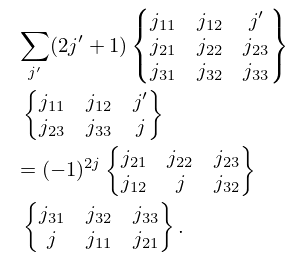
17: 34.7 Basic Properties: 9 ⁢ j Symbol

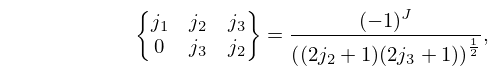
18: 34.5 Basic Properties: 6 ⁢ j Symbol

19: 10 Bessel Functions

20: 18 Orthogonal Polynomials

12: 34.6 Definition: $\mathit{9j}$ Symbol

$3j$ and $6j$ Symbols

15: 34.4 Definition: $\mathit{6j}$ Symbol

§34.4 Definition: $\mathit{6j}$ Symbol

17: 34.7 Basic Properties: $\mathit{9j}$ Symbol

18: 34.5 Basic Properties: $\mathit{6j}$ Symbol