.韩国兰芝岛世界杯公园_『网址:687.vii』篮球世界杯竞猜_b5p6v3_pr7bnb1nb.com

SearchAdvancedHelp

(0.005 seconds)

11—20 of 773 matching pages

11: 32.7 Bäcklund Transformations

… ►satisfies ${\text{P}}_{\text{V}}$ with … ►

§32.7(vii) Sixth Painlevé Equation

►Let $w_j(z_j)=w_j(z_j;{\alpha }_j,{\beta }_j,{\gamma }_j,{\delta }_j)$, $j=0,1,2,3$, be solutions of ${\text{P}}_{\text{VI}}$ with … ► ${\text{P}}_{\text{VI}}$ also has quadratic and quartic transformations. …Also, …

12: Bibliography Q

… ►

“Best possible” upper and lower bounds for the zeros of the Bessel function $J_{\nu }(x)$ . Trans. Amer. Math. Soc. 351 (7), pp. 2833–2859.

ⓘ

External Links:

ISSN 0002-9947, FullText, MathReview (Andrea Laforgia), ZentralBlatt

Referenced by:

§10.21(vii).

Encodings:

BibTeX

…

13: 8.17 Incomplete Beta Functions

… ►For a historical profile of ${\mathrm{B}}_x(a,b)$ see Dutka (1981). … ►where …The $4m$ and $4m+1$ convergents are less than $I_x(a,b)$, and the $4m+2$ and $4m+3$ convergents are greater than $I_x(a,b)$. … ►For $x>(a+1)/(a+b+2)$ or , more rapid convergence is obtained by computing $I_{1-x}(b,a)$ and using (8.17.4). … ►

§8.17(vii) Addendum to 8.17(i) Definitions and Basic Properties

…

14: Bibliography T

… ►

Asymptotic estimates of Stirling numbers. Stud. Appl. Math. 89 (3), pp. 233–243.

ⓘ

External Links:

ISSN 0022-2526, FullText, MathReview (E. Rodney Canfield), ZentralBlatt

Referenced by:

§26.8(vii).

Encodings:

BibTeX

… ►

High Speed Numerical Integration of Fermi Dirac Integrals. Master’s Thesis, Naval Postgraduate School, Monterey, CA.

ⓘ

External Links:

FullText

Referenced by:

§25.21(vii).

Encodings:

BibTeX

… ►

The Theory of Functions. 2nd edition, Oxford University Press, Oxford.

ⓘ

External Links:

ZentralBlatt

Referenced by:

§1.10(ix), §1.10(v), §1.8(i), §1.8(ii), §1.8(iii), §1.9(vii).

Encodings:

BibTeX

… ►

Numerical Linear Algebra. Society for Industrial and Applied Mathematics (SIAM), Philadelphia, PA.

ⓘ

External Links:

ISBN 0-89871-361-7, MathReview (Moody T. Chu), ZentralBlatt

Referenced by:

§3.2(iii), §3.2(vii).

Encodings:

BibTeX

… ►

Rational Chebyshev approximation for the Fermi-Dirac integral $F_{-3/2}(x)$ . Solid–State Electronics 41 (5), pp. 771–773.

ⓘ

External Links:

Document

Referenced by:

§25.21(vii).

Encodings:

BibTeX

…

15: 12.10 Uniform Asymptotic Expansions for Large Parameter

… ►These cases are treated in §§12.10(vii)–12.10(viii). … ►Higher polynomials $u_s(t)$ can be calculated from the recurrence relation …and the $v_s(t)$ then follow from … ►

§12.10(vii) Negative $a$, . Expansions in Terms of Airy Functions

… ►The coefficients $A_s(\zeta )$ and $B_s(\zeta )$ are given by …

16: 28.4 Fourier Series

… ►

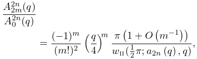
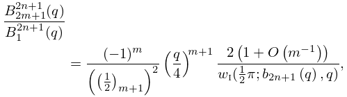
§28.4(vii) Asymptotic Forms for Large $m$

… ►

28.4.24 $$\frac{A_{2m}^{2n}(q)}{A_0^{2n}(q)}=\frac{{(-1)}^m}{{(m!)}^2}{\left(\frac{q}{4}\right)}^m\frac{\pi \left(1+O\left(m^{-1}\right)\right)}{w_{\text{II}}(\frac{1}{2}\pi ;a_{2n}\left(q\right),q)},$$

ⓘ

Symbols:

$O\left(x\right)$: order not exceeding, $a_n\left(q\right)$: eigenvalues of Mathieu equation, $\pi$: the ratio of the circumference of a circle to its diameter, $!$: factorial (as in $n!$), $m$: integer, $q=h^2$: parameter, $n$: integer, $w_{\text{II}}(z;a,q)$: fundamental solution and $A_m(q)$: Fourier coefficient

Permalink:

http://dlmf.nist.gov/28.4.E24

Encodings:

pMML, png, TeX

See also:

Annotations for §28.4(vii), §28.4 and Ch.28

►

28.4.25 $$\frac{A_{2m+1}^{2n+1}(q)}{A_1^{2n+1}(q)}=\frac{{(-1)}^{m+1}}{{\left({\left(\frac{1}{2}\right)}_{m+1}\right)}^2}{\left(\frac{q}{4}\right)}^{m+1}\frac{2\left(1+O\left(m^{-1}\right)\right)}{w_{\text{II}}^{\prime }(\frac{1}{2}\pi ;a_{2n+1}\left(q\right),q)},$$

ⓘ

Symbols:

$O\left(x\right)$: order not exceeding, $a_n\left(q\right)$: eigenvalues of Mathieu equation, ${\left(a\right)}_n$: Pochhammer’s symbol (or shifted factorial), $\pi$: the ratio of the circumference of a circle to its diameter, $m$: integer, $q=h^2$: parameter, $n$: integer, $w(z)$: Mathieu’s equation solution and $A_m(q)$: Fourier coefficient

Permalink:

http://dlmf.nist.gov/28.4.E25

Encodings:

pMML, png, TeX

See also:

Annotations for §28.4(vii), §28.4 and Ch.28

►

28.4.26 $$\frac{B_{2m+1}^{2n+1}(q)}{B_1^{2n+1}(q)}=\frac{{(-1)}^m}{{\left({\left(\frac{1}{2}\right)}_{m+1}\right)}^2}{\left(\frac{q}{4}\right)}^{m+1}\frac{2\left(1+O\left(m^{-1}\right)\right)}{w_{\text{I}}(\frac{1}{2}\pi ;b_{2n+1}\left(q\right),q)},$$

ⓘ

Symbols:

$O\left(x\right)$: order not exceeding, $b_n\left(q\right)$: eigenvalues of Mathieu equation, ${\left(a\right)}_n$: Pochhammer’s symbol (or shifted factorial), $\pi$: the ratio of the circumference of a circle to its diameter, $m$: integer, $q=h^2$: parameter, $n$: integer, $w_{\text{I}}(z;a,q)$: fundamental solution and $B_m(q)$: Fourier coefficient

Permalink:

http://dlmf.nist.gov/28.4.E26

Encodings:

pMML, png, TeX

See also:

Annotations for §28.4(vii), §28.4 and Ch.28

… ►For the basic solutions $w_{\text{I}}$ and $w_{\text{II}}$ see §28.2(ii).

17: 11.10 Anger–Weber Functions

… ►The Anger function ${𝐉}_{\nu }\left(z\right)$ and Weber function ${𝐄}_{\nu }\left(z\right)$ are defined by … ►The associated Anger–Weber function ${𝐀}_{\nu }\left(z\right)$ is defined by … ►

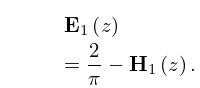
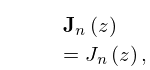
§11.10(vii) Special Values

… ►

11.10.26 ${𝐄}_0\left(z\right)=-{𝐇}_0\left(z\right),$ ${𝐄}_1\left(z\right)={\displaystyle \frac{2}{\pi }}-{𝐇}_1\left(z\right).$

ⓘ

Symbols:

${𝐇}_{\nu }\left(z\right)$: Struve function, ${𝐄}_{\nu }\left(z\right)$: Weber function, $\pi$: the ratio of the circumference of a circle to its diameter and $z$: complex variable

Referenced by:

§11.10(vii)

Permalink:

http://dlmf.nist.gov/11.10.E26

Encodings:

pMML, pMML, png, png, TeX, TeX

See also:

Annotations for §11.10(vii), §11.10 and Ch.11

… ►

11.10.29 $${𝐉}_n\left(z\right)=J_n\left(z\right),$$ $n\in \mathbb{Z}$.

ⓘ

Symbols:

${𝐉}_{\nu }\left(z\right)$: Anger function, $J_{\nu }\left(z\right)$: Bessel function of the first kind, $\in$: element of, $\mathbb{Z}$: set of all integers, $z$: complex variable and $n$: integer order

A&S Ref:

12.3.2

Referenced by:

§11.10(vii), §11.11(ii)

Permalink:

http://dlmf.nist.gov/11.10.E29

Encodings:

pMML, png, TeX

See also:

Annotations for §11.10(vii), §11.10 and Ch.11

…

18: 1.15 Summability Methods

… ► ${\int }_{-\mathrm{\infty }}^{\mathrm{\infty }}f(t)dt$ is Abel summable to $L$, or … ► ${\int }_{-\mathrm{\infty }}^{\mathrm{\infty }}f(t)dt$ is (C,1) summable to $L$, or … ►If ${\int }_{-\mathrm{\infty }}^{\mathrm{\infty }}f(t)dt$ converges and equals $L$, then the integral is Abel and Cesàro summable to $L$. … ►

§1.15(vii) Fractional Derivatives

… ►and either $\left|a_n\right|\le K$ or $a_n\ge 0$, then …

19: 13.2 Definitions and Basic Properties

… ►

§13.2(vii) Connection Formulas

… ►

13.2.39 $$M(a,b,z)={\mathrm{e}}^{z}M(b-a,b,-z),$$

ⓘ

Symbols:

$M(a,b,z)$: $={}_1{}^{}F_1^{}(a;b;z)$ Kummer confluent hypergeometric function, $\mathrm{e}$: base of natural logarithm and $z$: complex variable

A&S Ref:

13.1.27

Referenced by:

§13.12, §13.8(i), §13.9(ii), §18.17(vi)

Permalink:

http://dlmf.nist.gov/13.2.E39

Encodings:

pMML, png, TeX

See also:

Annotations for §13.2(vii), §13.2(vii), §13.2 and Ch.13

►

13.2.40 $$U(a,b,z)=z^{1-b}U(a-b+1,2-b,z).$$

ⓘ

Symbols:

$U(a,b,z)$: Kummer confluent hypergeometric function and $z$: complex variable

A&S Ref:

13.1.29

Referenced by:

§13.8(iii)

Permalink:

http://dlmf.nist.gov/13.2.E40

Encodings:

pMML, png, TeX

See also:

Annotations for §13.2(vii), §13.2(vii), §13.2 and Ch.13

►

13.2.41 $$\frac{1}{\mathrm{\Gamma }\left(b\right)}M(a,b,z)=\frac{{\mathrm{e}}^{\mp a\pi \mathrm{i}}}{\mathrm{\Gamma }\left(b-a\right)}U(a,b,z)+\frac{{\mathrm{e}}^{\pm (b-a)\pi \mathrm{i}}}{\mathrm{\Gamma }\left(a\right)}{\mathrm{e}}^{z}U(b-a,b,{\mathrm{e}}^{\pm \pi \mathrm{i}}z).$$

ⓘ

Symbols:

$\mathrm{\Gamma }\left(z\right)$: gamma function, $M(a,b,z)$: $={}_1{}^{}F_1^{}(a;b;z)$ Kummer confluent hypergeometric function, $U(a,b,z)$: Kummer confluent hypergeometric function, $\pi$: the ratio of the circumference of a circle to its diameter, $\mathrm{e}$: base of natural logarithm, $\mathrm{i}$: imaginary unit and $z$: complex variable

Referenced by:

§13.12, §13.14(vii), §13.4(i), §13.7(ii)

Permalink:

http://dlmf.nist.gov/13.2.E41

Encodings:

pMML, png, TeX

See also:

Annotations for §13.2(vii), §13.2(vii), §13.2 and Ch.13

… ►

13.2.42 $$U(a,b,z)=\frac{\mathrm{\Gamma }\left(1-b\right)}{\mathrm{\Gamma }\left(a-b+1\right)}M(a,b,z)+\frac{\mathrm{\Gamma }\left(b-1\right)}{\mathrm{\Gamma }\left(a\right)}{z}^{1-b}M(a-b+1,2-b,z).$$

ⓘ

Symbols:

$\mathrm{\Gamma }\left(z\right)$: gamma function, $M(a,b,z)$: $={}_1{}^{}F_1^{}(a;b;z)$ Kummer confluent hypergeometric function, $U(a,b,z)$: Kummer confluent hypergeometric function and $z$: complex variable

A&S Ref:

13.1.3 (in different form)

Referenced by:

§13.14(vii), §13.2(ii), §13.6(v), §13.9(ii), §33.13

Permalink:

http://dlmf.nist.gov/13.2.E42

Encodings:

pMML, png, TeX

See also:

Annotations for §13.2(vii), §13.2(vii), §13.2 and Ch.13

20: 34.3 Basic Properties: $\mathit{3}j$ Symbol

… ►When any one of $j_1,j_2,j_3$ is equal to $0,\frac{1}{2}$, or $1$, the $\mathit{3}j$ symbol has a simple algebraic form. …For these and other results, and also cases in which any one of $j_1,j_2,j_3$ is $\frac{3}{2}$ or $2$, see Edmonds (1974, pp. 125–127). … ►Even permutations of columns of a $\mathit{3}j$ symbol leave it unchanged; odd permutations of columns produce a phase factor ${(-1)}^{j_1+j_2+j_3}$, for example, … ►

§34.3(vii) Relations to Legendre Polynomials and Spherical Harmonics

►For the polynomials $P_l$ see §18.3, and for the function $Y_{l,m}$ see §14.30. …