.%E9%9F%A9%E5%9B%BD%E5%85%B0%E8%8A%9D%E5%B2%9B%E4%B8%96%E7%95%8C%E6%9D%AF%E5%85%AC%E5%9B%AD_%E3%80%8E%E7%BD%91%E5%9D%80%3A68707.vip%E3%80%8F%E7%AF%AE%E7%90%83%E4%B8%96%E7%95%8C%E6%9D%AF%E7%AB%9E%E7%8C%9C_b5p6v3_pr7bnb1nb.com
(0.075 seconds)
21—30 of 848 matching pages
21: 10 Bessel Functions
…
22: 23 Weierstrass Elliptic and Modular
Functions
…
23: 19.5 Maclaurin and Related Expansions
…
►where is the Gauss hypergeometric function (§§15.1 and 15.2(i)).
…where is an Appell function (§16.13).
…
►Coefficients of terms up to are given in Lee (1990), along with tables of fractional errors in and , , obtained by using 12 different truncations of (19.5.6) in (19.5.8) and (19.5.9).
…
►Series expansions of and are surveyed and improved in Van de Vel (1969), and the case of is summarized in Gautschi (1975, §1.3.2).
For series expansions of when see Erdélyi et al. (1953b, §13.6(9)).
…
24: 34.8 Approximations for Large Parameters
§34.8 Approximations for Large Parameters
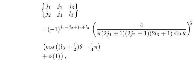
►For large values of the parameters in the , , and symbols, different asymptotic forms are obtained depending on which parameters are large. … ►
34.8.1
,
…
►Uniform approximations in terms of Airy functions for the and symbols are given in Schulten and Gordon (1975b).
For approximations for the , , and symbols with error bounds see Flude (1998), Chen et al. (1999), and Watson (1999): these references also cite earlier work.
25: 7.8 Inequalities
…
►
7.8.1
…
►
7.8.5
.
…
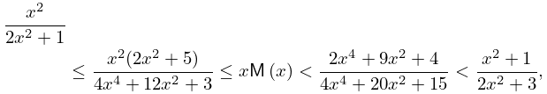
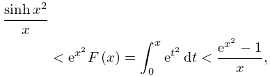
►
7.8.7
.
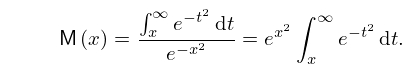
►The function is strictly decreasing for .
For these and similar results for Dawson’s integral see Janssen (2021).
…
26: 4.25 Continued Fractions
27: 19.36 Methods of Computation
…
►For the polynomial of degree 7, for example, is
…
►
can be evaluated by using (19.25.5).
…Thompson (1997, pp. 499, 504) uses descending Landen transformations for both and .
A summary for is given in Gautschi (1975, §3).
…
►Similarly, §19.26(ii) eases the computation of functions such as when () is small compared with .
…
28: 18.26 Wilson Class: Continued
…
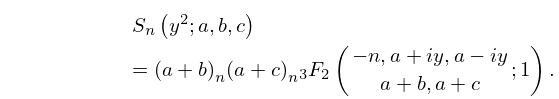
►Here we use as convention for (16.2.1) with , , and that the summation on the right-hand side ends at .
…
►
18.26.2
…
►For comments on the use of the forward-difference operator , the backward-difference operator , and the central-difference operator , see §18.2(ii).
…
►See Koekoek et al. (2010, Chapter 9) for further formulas.
…
►For the hypergeometric function see §§15.1 and 15.2(i).
…
29: 15.12 Asymptotic Approximations
…
►For the asymptotic behavior of as with , , fixed, combine (15.2.2) with (15.8.2) or (15.8.8).
…
►
(d)
…
►where and , , are defined by the generating function
…
►For see §10.25(ii).
…
►By combination of the foregoing results of this subsection with the linear transformations of §15.8(i) and the connection formulas of §15.10(ii), similar asymptotic approximations for can be obtained with or , .
…
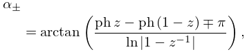
and , where
15.12.1
with restricted so that .
30: 18 Orthogonal Polynomials
…
