DLMF: Untitled Document

… ►

See accompanying text — Figure 23.4.1: $\wp\left(x;g_{2},0\right)$ for $0\leq x\leq 9$ , $g_{2}$ = 0. …8. … Magnify

►

… ►

…

§34.12 Physical Applications

►The angular momentum coupling coefficients (

\mathit{3j}

,

\mathit{6j}

, and

\mathit{9j}

symbols) are essential in the fields of nuclear, atomic, and molecular physics. …

\mathit{3j},\mathit{6j}

, and

\mathit{9j}

symbols are also found in multipole expansions of solutions of the Laplace and Helmholtz equations; see Carlson and Rushbrooke (1950) and Judd (1976).

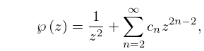
… ►An algebraic curve that can be put either into the form … ►It follows from the addition formula (23.10.1) that the points

P_{j}=P(z_{j})

,

j=1,2,3

, have zero sum iff

z_{1}+z_{2}+z_{3}\in\mathbb{L}

, so that addition of points on the curve

C

corresponds to addition of parameters

z_{j}

on the torus

\mathbb{C}/\mathbb{L}

; see McKean and Moll (1999, §§2.11, 2.14). … ►The addition law states that to find the sum of two points, take the third intersection with

C

of the chord joining them (or the tangent if they coincide); then its reflection in the

x

-axis gives the required sum. … ►Both

T, K

are subgroups of

C

, though

I

may not be. …The order of a point (if finite and not already determined) can have only the values 3, 5, 6, 7, 9, 10, or 12, and so can be found from

2P=-P

,

4P=-P

,

4P=-2P

,

8P=P

,

8P=-P

,

8P=-2P

, or

8P=-4P

. …

… ►

23.9.1

c_{n}=(2n-1)\sum_{w\in\mathbb{L}\setminus\{0\}}w^{-2n},

n=2,3,4,\dots

.

ⓘ

Symbols:: $\in$ : element of, $\setminus$ : set subtraction, $\mathbb{L}$ : lattice, $n$ : integer and $c_{n}$
Referenced by:: §20.6
Permalink:: http://dlmf.nist.gov/23.9.E1
Encodings:: pMML, png, TeX
See also:: Annotations for §23.9 and Ch.23

… ►

23.9.2

\wp\left(z\right)=\frac{1}{z^{2}}+\sum_{n=2}^{\infty}c_{n}z^{2n-2},

0<|z|<|z_{0}|

,

ⓘ

Symbols:: $\wp\left(\NVar{z}\right)$ (= $\wp\left(z|\mathbb{L}\right)$ = $\wp\left(z;g_{2},g_{3}\right)$ ): Weierstrass $\wp$ -function, $\mathbb{L}$ : lattice, $n$ : integer, $z$ : complex and $c_{n}$
A&S Ref:: 18.5.1
Referenced by:: §23.9, §23.9
Permalink:: http://dlmf.nist.gov/23.9.E2
Encodings:: pMML, png, TeX
See also:: Annotations for §23.9 and Ch.23

… ►Explicit coefficients

c_{n}

in terms of

c_{2}

and

c_{3}

are given up to

c_{19}

in Abramowitz and Stegun (1964, p. 636). ►For

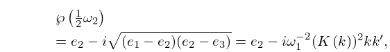
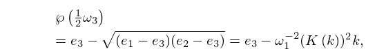
j=1,2,3

, and with

e_{j}

as in §23.3(i), … ►For

a_{m,n}

with

m=0,1,\dots,12

and

n=0,1,\dots,8

, see Abramowitz and Stegun (1964, p. 637).

… ►

23.7.1

\wp\left(\tfrac{1}{2}\omega_{1}\right)=e_{1}+\sqrt{(e_{1}-e_{3})(e_{1}-e_{2})}% =e_{1}+\omega_{1}^{-2}(K\left(k\right))^{2}k^{\prime},

ⓘ

Symbols:: $\wp\left(\NVar{z}\right)$ (= $\wp\left(z|\mathbb{L}\right)$ = $\wp\left(z;g_{2},g_{3}\right)$ ): Weierstrass $\wp$ -function, $e_{\NVar{j}}$ : Weierstrass lattice roots, $K\left(\NVar{k}\right)$ : Legendre’s complete elliptic integral of the first kind, $\mathbb{L}$ : lattice, $\omega_{1}$ , $\omega_{3}$ , $\omega_{2}=-\omega_{1}-\omega_{3}$ : lattice generators, $k$ : modulus and $k^{\prime}$ : complementary modulus
A&S Ref:: 18.3.18
Permalink:: http://dlmf.nist.gov/23.7.E1
Encodings:: pMML, png, TeX
See also:: Annotations for §23.7 and Ch.23

►

23.7.2

\wp\left(\tfrac{1}{2}\omega_{2}\right)=e_{2}-i\sqrt{(e_{1}-e_{2})(e_{2}-e_{3})% }=e_{2}-i\omega_{1}^{-2}(K\left(k\right))^{2}kk^{\prime},

ⓘ

Symbols:: $\wp\left(\NVar{z}\right)$ (= $\wp\left(z|\mathbb{L}\right)$ = $\wp\left(z;g_{2},g_{3}\right)$ ): Weierstrass $\wp$ -function, $e_{\NVar{j}}$ : Weierstrass lattice roots, $K\left(\NVar{k}\right)$ : Legendre’s complete elliptic integral of the first kind, $\mathrm{i}$ : imaginary unit, $\mathbb{L}$ : lattice, $\omega_{1}$ , $\omega_{3}$ , $\omega_{2}=-\omega_{1}-\omega_{3}$ : lattice generators, $k$ : modulus and $k^{\prime}$ : complementary modulus
A&S Ref:: 18.3.18
Permalink:: http://dlmf.nist.gov/23.7.E2
Encodings:: pMML, png, TeX
See also:: Annotations for §23.7 and Ch.23

►

23.7.3

\wp\left(\tfrac{1}{2}\omega_{3}\right)=e_{3}-\sqrt{(e_{1}-e_{3})(e_{2}-e_{3})}% =e_{3}-\omega_{1}^{-2}(K\left(k\right))^{2}k,

ⓘ

Symbols:: $\wp\left(\NVar{z}\right)$ (= $\wp\left(z|\mathbb{L}\right)$ = $\wp\left(z;g_{2},g_{3}\right)$ ): Weierstrass $\wp$ -function, $e_{\NVar{j}}$ : Weierstrass lattice roots, $K\left(\NVar{k}\right)$ : Legendre’s complete elliptic integral of the first kind, $\mathbb{L}$ : lattice, $\omega_{1}$ , $\omega_{3}$ , $\omega_{2}=-\omega_{1}-\omega_{3}$ : lattice generators and $k$ : modulus
A&S Ref:: 18.3.18
Permalink:: http://dlmf.nist.gov/23.7.E3
Encodings:: pMML, png, TeX
See also:: Annotations for §23.7 and Ch.23

…

… ►

S. Lai and Y. Chiu (1992) Exact computation of the

9

-

j

symbols. Comput. Phys. Comm. 70 (3), pp. 544–556.

ⓘ

Notes:: Double-precision Fortran
External Links:: ISSN 0010-4655, Document, Code, MathReview
Referenced by:: 7th item.
Encodings:: BibTeX

… ►

E. M. Lifshitz and L. P. Pitaevskiĭ (1980) Statistical Physics, Part 2: Theory of the Condensed State. Pergamon Press, Oxford.

ⓘ

Notes:: Course of Theoretical Physics , Vol. 9. Translated from the Russian by J. B. Sykes and M. J. Kearsley.
External Links:: ISBN 0-08-023073-3; 0-08-023072-5, MathReview
Referenced by:: §25.17.
Encodings:: BibTeX

… ►

J. L. López, P. Pagola, and E. Pérez Sinusía (2013b) Asymptotics of the first Appell function

F_{1}

with large parameters. Integral Transforms Spec. Funct. 24 (9), pp. 715–733.

ⓘ

External Links:: ISSN 1065-2469, Document, FullText, MathReview Entry, ZentralBlatt
Referenced by:: §16.13, §16.13.
Encodings:: BibTeX

… ►

L. Lorch and P. Szegő (1964) Monotonicity of the differences of zeros of Bessel functions as a function of order. Proc. Amer. Math. Soc. 15 (1), pp. 91–96.

ⓘ

External Links:: ISSN 0002-9939, FullText, MathReview (F. W. J. Olver), ZentralBlatt
Referenced by:: §10.21(ii).
Encodings:: BibTeX

… ►

Lord Kelvin (1905) Deep water ship-waves. Phil. Mag. 9, pp. 733–757.

ⓘ

External Links:: ZentralBlatt
Referenced by:: §36.13.
Encodings:: BibTeX

…

… ►

H. E. Salzer (1955) Orthogonal polynomials arising in the numerical evaluation of inverse Laplace transforms. Math. Tables Aids Comput. 9 (52), pp. 164–177.

ⓘ

External Links:: FullText, MathReview (S. C. van Veen), ZentralBlatt
Referenced by:: §3.5(viii).
Encodings:: BibTeX

… ►

J. Segura and A. Gil (1999) Evaluation of associated Legendre functions off the cut and parabolic cylinder functions. Electron. Trans. Numer. Anal. 9, pp. 137–146.

ⓘ

Notes:: Orthogonal polynomials: numerical and symbolic algorithms (Leganés, 1998)
External Links:: ISSN 1068-9613, FullText, MathReview (Adam Marlewski), ZentralBlatt
Referenced by:: §14.30(i), 3rd item.
Encodings:: BibTeX

… ►

G. Shanmugam (1978) Parabolic Cylinder Functions and their Application in Symmetric Two-centre Shell Model. In Proceedings of the Conference on Mathematical Analysis and its Applications (Inst. Engrs., Mysore, 1977), Matscience Rep., Vol. 91, Aarhus, pp. P81–P89.

ⓘ

External Links:: MathReview
Referenced by:: §12.17.
Encodings:: BibTeX

… ►

K. Srinivasa Rao, V. Rajeswari, and C. B. Chiu (1989) A new Fortran program for the

9

-

j

angular momentum coefficient. Comput. Phys. Comm. 56 (2), pp. 231–248.

ⓘ

External Links:: Document, ZentralBlatt
Referenced by:: §34.13.
Encodings:: BibTeX

… ►

S. K. Suslov (2003) An Introduction to Basic Fourier Series. Developments in Mathematics, Vol. 9, Kluwer Academic Publishers, Dordrecht.

ⓘ

External Links:: ISBN 1-4020-1221-7, MathReview (P. D. F. Ion), ZentralBlatt
Referenced by:: §17.3(i).
Encodings:: BibTeX

…

… ►and are denoted by

e_{1},e_{2},e_{3}

. … ►Let

{g_{2}}^{3}\neq 27{g_{3}}^{2}

, or equivalently

\Delta

be nonzero, or

e_{1},e_{2},e_{3}

be distinct. Given

g_{2}

and

g_{3}

there is a unique lattice

\mathbb{L}

such that (23.3.1) and (23.3.2) are satisfied. … ►Conversely,

g_{2}

,

g_{3}

, and the set

\{e_{1},e_{2},e_{3}\}

are determined uniquely by the lattice

\mathbb{L}

independently of the choice of generators. However, given any pair of generators

2\omega_{1}

,

2\omega_{3}

of

\mathbb{L}

, and with

\omega_{2}

defined by (23.2.1), we can identify the

e_{j}

individually, via …

… ►

I. G. Macdonald (1972) Affine root systems and Dedekind’s

\eta

-function. Invent. Math. 15 (2), pp. 91–143.

ⓘ

External Links:: Document, MathReview (D.-N. Verma), ZentralBlatt
Referenced by:: §20.12(i).
Encodings:: BibTeX

… ►

J. McMahon (1894) On the roots of the Bessel and certain related functions. Ann. of Math. 9 (1-6), pp. 23–30.

ⓘ

External Links:: ISSN 0003-486X, FullText, MathReview Entry, ZentralBlatt
Referenced by:: §10.21(x).
Encodings:: BibTeX

… ►

J. Meixner (1934) Orthogonale Polynomsysteme mit einer besonderen Gestalt der erzeugenden Funktion. J. Lond. Math. Soc. 9, pp. 6–13 (German).

ⓘ

External Links:: ISSN 0024-6107; 1469-7750/e, ZentralBlatt
Referenced by:: §18.2(xii).
Encodings:: BibTeX

… ►

S. C. Milne and G. M. Lilly (1992) The

A_{l}

and

C_{l}

Bailey transform and lemma. Bull. Amer. Math. Soc. (N.S.) 26 (2), pp. 258–263.

ⓘ

External Links:: ISSN 0273-0979, Pdf, Document, MathReview (Robert A. Gustafson), ZentralBlatt
Referenced by:: §17.12.
Encodings:: BibTeX

… ►

T. Morita (2013) A connection formula for the

q

-confluent hypergeometric function. SIGMA Symmetry Integrability Geom. Methods Appl. 9, pp. Paper 050, 13.

ⓘ

External Links:: ISSN 1815-0659, Document, MathReview (Jeremy Lovejoy), ZentralBlatt
Referenced by:: §17.6(ii), §17.6(ii).
Encodings:: BibTeX

…

… ►

R. G. Campos (1995) A quadrature formula for the Hankel transform. Numer. Algorithms 9 (2), pp. 343–354.

ⓘ

External Links:: ISSN 1017-1398, Document, MathReview (V. I. Polovinkin), ZentralBlatt
Referenced by:: §10.74(vii).
Encodings:: BibTeX

… ►

B. C. Carlson (1978) Short proofs of three theorems on elliptic integrals. SIAM J. Math. Anal. 9 (3), pp. 524–528.

ⓘ

External Links:: Document, MathReview (Y. L. Luke), ZentralBlatt
Referenced by:: §19.26(i).
Encodings:: BibTeX

… ►

T. S. Chihara and M. E. H. Ismail (1993) Extremal measures for a system of orthogonal polynomials. Constr. Approx. 9, pp. 111–119.

ⓘ

External Links:: ISSN 0176-4276, Document, MathReview (Mizan Rahman), ZentralBlatt
Referenced by:: §18.28(iv).
Encodings:: BibTeX

… ►

J. S. Christiansen and M. E. H. Ismail (2006) A moment problem and a family of integral evaluations. Trans. Amer. Math. Soc. 358 (9), pp. 4071–4097.

ⓘ

External Links:: ISSN 0002-9947, Document, MathReview (Roelof Koekoek), ZentralBlatt
Referenced by:: §18.28(iv).
Encodings:: BibTeX

… ►

Th. Clausen (1828) Über die Fälle, wenn die Reihe von der Form

y=1+\frac{\alpha}{1}\cdot\frac{\beta}{\gamma}x+\frac{\alpha\cdot\alpha+1}{1% \cdot 2}\cdot\frac{\beta\cdot\beta+1}{\gamma\cdot\gamma+1}x^{2}+

etc. ein Quadrat von der Form

z=1+\frac{\alpha^{\prime}}{1}\cdot\frac{\beta^{\prime}}{\gamma^{\prime}}\cdot% \frac{\delta^{\prime}}{\epsilon^{\prime}}x+\frac{\alpha^{\prime}\cdot\alpha^{% \prime}+1}{1\cdot 2}\cdot\frac{\beta^{\prime}\cdot\beta^{\prime}+1}{\gamma^{% \prime}\cdot\gamma^{\prime}+1}\cdot\frac{\delta^{\prime}\cdot\delta^{\prime}+1% }{\epsilon^{\prime}\cdot\epsilon^{\prime}+1}x^{2}+

etc. hat. J. Reine Angew. Math. 3, pp. 89–91.

ⓘ

External Links:: Link, MathReview Entry, ZentralBlatt
Referenced by:: §16.12.
Encodings:: BibTeX

…

.%E7%BD%91%E7%BB%9C%E7%9B%B4%E6%92%AD%E4%B8%96%E7%95%8C%E6%9D%AFapp%E3%80%8E%E7%BD%91%E5%9D%80%3Amxsty.cc%E3%80%8F.2022%E4%B8%8B%E5%B1%8A%E4%B8%96%E7%95%8C%E6%9D%AF%E5%9C%A8%E5%93%AA%E4%B8%AA%E5%9B%BD%E5%AE%B6-m6q3s2-2022%E5%B9%B411%E6%9C%8829%E6%97%A56%E6%97%B623%E5%88%8616%E7%A7%92wmcsgwckm.com

21—30 of 751 matching pages

21: 23.4 Graphics

22: 34.12 Physical Applications

§34.12 Physical Applications

23: 23.20 Mathematical Applications

24: 23.9 Laurent and Other Power Series

25: 23.7 Quarter Periods

26: Bibliography L

27: Bibliography S

28: 23.3 Differential Equations

29: Bibliography M

30: Bibliography C