.%E5%8D%A1%E5%A1%94%E5%B0%94%E4%B8%96%E7%95%8C%E6%9D%AF%E5%A5%96%E9%87%91_%E3%80%8E%E7%BD%91%E5%9D%80%3A68707.vip%E3%80%8F%E4%B8%96%E7%95%8C%E6%9D%AF%E7%AB%9E%E7%8C%9C_b5p6v3_2022%E5%B9%B411%E6%9C%8830%E6%97%A521%E6%97%B649%E5%88%8653%E7%A7%92_3vjzhlfvb.cc

SearchAdvancedHelp

(0.038 seconds)

21—30 of 720 matching pages

21: 19.1 Special Notation

… ►We use also the function $D(\varphi ,k)$, introduced by Jahnke et al. (1966, p. 43). … ►In Abramowitz and Stegun (1964, Chapter 17) the functions (19.1.1) and (19.1.2) are denoted, in order, by $K(\alpha )$, $E(\alpha )$, $\mathrm{\Pi }(n\backslash \alpha )$, $F(\varphi \backslash \alpha )$, $E(\varphi \backslash \alpha )$, and $\mathrm{\Pi }(n;\varphi \backslash \alpha )$, where $\alpha =\arcsin k$ and $n$ is the ${\alpha }^2$ (not related to $k$) in (19.1.1) and (19.1.2). …However, it should be noted that in Chapter 8 of Abramowitz and Stegun (1964) the notation used for elliptic integrals differs from Chapter 17 and is consistent with that used in the present chapter and the rest of the NIST Handbook and DLMF. … ►

$R_D(x,y,z)$ ,

… ► $R_F(x,y,z)$, $R_G(x,y,z)$, and $R_J(x,y,z,p)$ are the symmetric (in $x$, $y$, and $z$) integrals of the first, second, and third kinds; they are complete if exactly one of $x$, $y$, and $z$ is identically 0. …

22: 31.2 Differential Equations

… ►where $2{\omega }_1$ and $2{\omega }_3$ with $\mathrm{\Im }\left({\omega }_3/{\omega }_1\right)>0$ are generators of the lattice $𝕃$ for $\mathrm{\wp }\left(z|𝕃\right)$. … ►

$F$-Homotopic Transformations

… ►By composing these three steps, there result $2^3=8$ possible transformations of the dependent variable (including the identity transformation) that preserve the form of (31.2.1). … ►There are $4!=24$ homographies $\tilde{z}(z)=(Az+B)/(Cz+D)$ that take $0,1,a,\mathrm{\infty }$ to some permutation of $0,1,a^{\prime },\mathrm{\infty }$, where $a^{\prime }$ may differ from $a$. … ►There are $8\cdot 24=192$ automorphisms of equation (31.2.1) by compositions of $F$-homotopic and homographic transformations. …

23: 1.18 Linear Second Order Differential Operators and Eigenfunction Expansions

… ►Assume that $𝒟(T)$ is dense in $V$, i. … ► $u_{\lambda }\in 𝒟(T)$, corresponding to distinct eigenvalues, are orthogonal: i. … ►This insures the vanishing of the boundary terms in (1.18.26), and also is a choice which indicates that $𝒟(T)=𝒟(T^{\ast })$, as $f(x)$ and $g(x)$ satisfy the same boundary conditions and thus define the same domains. … ►, $𝒟(T)\subset 𝒟(T^{\ast })$ and $T^{\ast }v=Tv$ for $v\in 𝒟(T)$. … ►Let $T$ be a linear operator on $V$ with dense domain $𝒟(T)$ and with range $ℛ(T)=\{Tv\mid v\in 𝒟(T)\}$. …

24: 10.70 Zeros

… ►

10.70.1 $$\frac{\mu -1}{16t}+\frac{\mu -1}{32t^2}+\frac{(\mu -1)(5\mu +19)}{1536t^3}+\frac{3{(\mu -1)}^2}{512t^4}+\mathrm{\cdots }.$$

ⓘ

Defines:

$f(t)$: function (locally)

A&S Ref:

9.10.35

Referenced by:

§10.70

Permalink:

http://dlmf.nist.gov/10.70.E1

Encodings:

pMML, png, TeX

See also:

Annotations for §10.70 and Ch.10

… ►

$$\text{zeros of }{\mathrm{ber}}_{\nu }x\sim \sqrt{2}(t-f(t)),$$ $t=(m-\frac{1}{2}\nu -\frac{3}{8})\pi$,

►

$$\text{zeros of }{\mathrm{bei}}_{\nu }x\sim \sqrt{2}(t-f(t)),$$ $t=(m-\frac{1}{2}\nu +\frac{1}{8})\pi$,

►

$$\text{zeros of }{\ker }_{\nu }x\sim \sqrt{2}(t+f(-t)),$$ $t=(m-\frac{1}{2}\nu -\frac{5}{8})\pi$,

►

$$\text{zeros of }{\mathrm{kei}}_{\nu }x\sim \sqrt{2}(t+f(-t)),$$ $t=(m-\frac{1}{2}\nu -\frac{1}{8})\pi$.

…

25: 16.25 Methods of Computation

… ►See §§3.6(vii), 3.7(iii), Olde Daalhuis and Olver (1998), Lozier (1980), and Wimp (1984, Chapters 7, 8).

26: 20 Theta Functions

…

27: 36 Integrals with Coalescing Saddles

…

28: 19.17 Graphics

… ►For $R_F$, $R_G$, and $R_J$, which are symmetric in $x,y,z$, we may further assume that $z$ is the largest of $x,y,z$ if the variables are real, then choose $z=1$, and consider only $0\le x\le 1$ and $0\le y\le 1$. … ►To view $R_F(0,y,1)$ and $2R_G(0,y,1)$ for complex $y$, put $y=1-k^2$, use (19.25.1), and see Figures 19.3.7–19.3.12. … ►To view $R_F(0,y,1)$ and $2R_G(0,y,1)$ for complex $y$, put $y=1-k^2$, use (19.25.1), and see Figures 19.3.7–19.3.12. … ►

►►

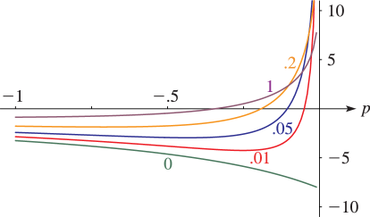
Figure 19.17.7: Cauchy principal value of $R_J(0.5,y,1,p)$ for $y=0,\mathrm{\hspace{0.17em}0.01},\mathrm{\hspace{0.17em}0.05},\mathrm{\hspace{0.17em}0.2},\mathrm{\hspace{0.17em}1}$, . $y=1$ corresponds to $3(R_C(0.5,p)-(\pi /\sqrt{8}))/(1-p)$. … Magnify

►

►

►

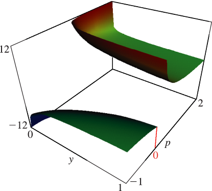
Figure 19.17.8: $R_J(0,y,1,p)$, $0\le y\le 1$, $-1\le p\le 2$. …When $p=1$, it reduces to $R_D(0,y,1)$. … Magnify 3D Help

29: Bibliography L

… ►

On the maxima and minima of Bernoulli polynomials. Amer. Math. Monthly 47 (8), pp. 533–538.

ⓘ

External Links:

FullText, MathReview (W. E. Milne), ZentralBlatt

Referenced by:

§24.12(i), §24.9.

Encodings:

BibTeX

… ►

A partition function connected with the modulus five. Duke Math. J. 8 (4), pp. 631–655.

ⓘ

External Links:

Document, MathReview (R. D. James), ZentralBlatt

Referenced by:

§17.18.

Encodings:

BibTeX

… ►

Algorithm 567: Extended-range arithmetic and normalized Legendre polynomials [A1], [C1]. ACM Trans. Math. Software 7 (1), pp. 141–146.

ⓘ

Notes:

Double-precision Fortran, minumum accuracy 13S

External Links:

ISSN 0098-3500, Document, GAMS (module 567; package TOMS)

Referenced by:

6th item.

Encodings:

BibTeX

… ►

Solutions of the fifth Painlevé equation. Differ. Uravn. 4 (8), pp. 1413–1420 (Russian).

ⓘ

Notes:

In Russian. English translation: Differential Equations 4(8), pp. 732–735

External Links:

MathReview (C. E. Langenhop), ZentralBlatt

Referenced by:

§32.10(v), §32.8(v).

Encodings:

BibTeX

… ►

Miniaturized tables of Bessel functions. II. Math. Comp. 25 (116), pp. 789–795 and D14–E13.

ⓘ

Notes:

For Corrigendum see same journal 26(120), pp. A1–A7

External Links:

ISSN 0025-5718, FullText, MathReview, ZentralBlatt

Referenced by:

§10.76(ii).

Encodings:

BibTeX

…

30: 3.3 Interpolation

… ►If $f$ is analytic in a simply-connected domain $D$ (§1.13(i)), then for $z\in D$, …where $C$ is a simple closed contour in $D$ described in the positive rotational sense and enclosing the points $z,z_1,z_2,\mathrm{\dots },z_n$. … ►If $f$ is analytic in a simply-connected domain $D$, then for $z\in D$, …where ${\omega }_{n+1}(\zeta )$ is given by (3.3.3), and $C$ is a simple closed contour in $D$ described in the positive rotational sense and enclosing $z_0,z_1,\mathrm{\dots },z_n$. … ►Then by using $x_3$ in Newton’s interpolation formula, evaluating $\left[x_0,x_1,x_2,x_3\right]f=-\mathrm{0.26608\hspace{0.33em}28233}$ and recomputing $f^{\prime }(x)$, another application of Newton’s rule with starting value $x_3$ gives the approximation $x=\mathrm{2.33810\hspace{0.33em}7373}$, with 8 correct digits. …