👉1(716)351-6210📞Delta Flights 🪐Airlines 🛸flight cancellation
(0.003 seconds)
11—20 of 823 matching pages
11: 4.17 Special Values and Limits
12: 3.5 Quadrature
…
►where .
…
►with , , and .
…with , and .
…
►We choose so that at infinity.
…
►with saddle point at , and when the vertical path intersects the real axis at the saddle point.
…
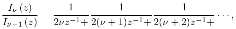
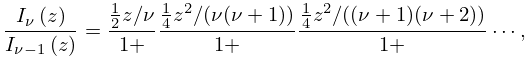
13: 13.29 Methods of Computation
…
►In the sector the integration has to be towards the origin, with starting values computed from asymptotic expansions (§§13.7 and 13.19).
On the rays , integration can proceed in either direction.
…
►
Example 1
►We assume . … ►We assume . …14: 18.31 Bernstein–Szegő Polynomials
…
►Let be a polynomial of degree and positive when .
The Bernstein–Szegő polynomials
, , are orthogonal on with respect to three types of weight function: , , .
In consequence, can be given explicitly in terms of and sines and cosines, provided that in the first case, in the second case, and in the third case.
…
15: 26.4 Lattice Paths: Multinomial Coefficients and Set Partitions
…
►For , the multinomial coefficient is defined to be .
…
►
is the multinominal coefficient (26.4.2):
… is the number of permutations of with cycles of length 1, cycles of length 2, , and cycles of length :
… is the number of set partitions of with subsets of size 1, subsets of size 2, , and subsets of size :
…For each all possible values of are covered.
…
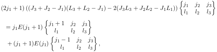
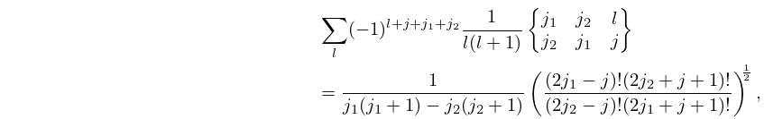
16: 34.5 Basic Properties: Symbol
…
►If any lower argument in a symbol is , , or , then the symbol has a simple algebraic form.
…
►
34.5.4
…
►
34.5.11
…
►
34.5.18
…
►
34.5.22
.
…
17: 24.20 Tables
…
►Abramowitz and Stegun (1964, Chapter 23) includes exact values of , , ; , , , , 20D; , , 18D.
…
►For information on tables published before 1961 see Fletcher et al. (1962, v. 1, §4) and Lebedev and Fedorova (1960, Chapters 11 and 14).
