��V��ATV1819��e3y6

(0.001 seconds)

21—30 of 69 matching pages

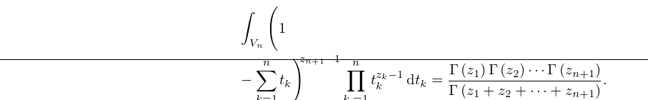
21: 5.14 Multidimensional Integrals

… ►Let

V_{n}

be the simplex:

t_{1}+t_{2}+\dots+t_{n}\leq 1

t_{k}\geq 0

. … ►

5.14.1

\int_{V_{n}}t_{1}^{z_{1}-1}t_{2}^{z_{2}-1}\cdots t_{n}^{z_{n}-1}\,\mathrm{d}t_% {1}\,\mathrm{d}t_{2}\cdots\,\mathrm{d}t_{n}=\frac{\Gamma\left(z_{1}\right)% \Gamma\left(z_{2}\right)\cdots\Gamma\left(z_{n}\right)}{\Gamma\left(1+z_{1}+z_% {2}+\dots+z_{n}\right)},

ⓘ

Symbols:: $\Gamma\left(\NVar{z}\right)$ : gamma function, $\,\mathrm{d}\NVar{x}$ : differential of $x$ , $\int$ : integral, $n$ : nonnegative integer, $z$ : complex variable and $V_{n}$ : simplex
Referenced by:: §5.19(iii)
Permalink:: http://dlmf.nist.gov/5.14.E1
Encodings:: pMML, png, TeX
See also:: Annotations for §5.14 and Ch.5

►

5.14.2

\int_{V_{n}}\left(1-\sum_{k=1}^{n}t_{k}\right)^{z_{n+1}-1}\prod_{k=1}^{n}t_{k}% ^{z_{k}-1}\,\mathrm{d}t_{k}=\frac{\Gamma\left(z_{1}\right)\Gamma\left(z_{2}% \right)\cdots\Gamma\left(z_{n+1}\right)}{\Gamma\left(z_{1}+z_{2}+\dots+z_{n+1}% \right)}.

ⓘ

Symbols:: $\Gamma\left(\NVar{z}\right)$ : gamma function, $\,\mathrm{d}\NVar{x}$ : differential of $x$ , $\int$ : integral, $n$ : nonnegative integer, $k$ : nonnegative integer, $z$ : complex variable and $V_{n}$ : simplex
Referenced by:: §5.19(iii)
Permalink:: http://dlmf.nist.gov/5.14.E2
Encodings:: pMML, png, TeX
See also:: Annotations for §5.14 and Ch.5

…

22: 12.1 Special Notation

… ►The main functions treated in this chapter are the parabolic cylinder functions (PCFs), also known as Weber parabolic cylinder functions:

U\left(a,z\right)

V\left(a,z\right)

\overline{U}\left(a,z\right)

, and

W\left(a,z\right)

. …

23: 18.7 Interrelations and Limit Relations

… ►

18.7.5

V_{n}\left(x\right)=\ifrac{P^{(-\frac{1}{2},\frac{1}{2})}_{n}\left(x\right)}{P% ^{(-\frac{1}{2},\frac{1}{2})}_{n}\left(1\right)},

ⓘ

Symbols:: $W_{\NVar{n}}\left(\NVar{x}\right)$ : Chebyshev polynomial of the fourth kind, $V_{\NVar{n}}\left(\NVar{x}\right)$ : Chebyshev polynomial of the third kind, $P^{(\NVar{\alpha},\NVar{\beta})}_{\NVar{n}}\left(\NVar{x}\right)$ : Jacobi polynomial, $n$ : nonnegative integer and $x$ : real variable
Referenced by:: §18.17(viii), §18.5(i), (18.7.5), (18.7.6), §18.7(i), §18.7(ii), Erratum (V1.0.28) for Table 18.3.1
Permalink:: http://dlmf.nist.gov/18.7.E5
Encodings:: pMML, png, TeX
Correction (effective with 1.0.28):: The DLMF now adopts the definitions for the Chebyshev polynomials of the third and fourth kinds $V_{n}\left(x\right)$ , $W_{n}\left(x\right)$ used in Mason and Handscomb (2003). Therefore $V_{n}\left(x\right)$ , $W_{n}\left(x\right)$ , having been interchanged, the right-hand sides of (18.7.5) and (18.7.6) have been interchanged. For further details see Errata.
See also:: Annotations for §18.7(i), §18.7(i), §18.7 and Ch.18

►

18.7.6

W_{n}\left(x\right)=\ifrac{(2n+1)P^{(\frac{1}{2},-\frac{1}{2})}_{n}\left(x% \right)}{P^{(\frac{1}{2},-\frac{1}{2})}_{n}\left(1\right)}.

ⓘ

Symbols:: $W_{\NVar{n}}\left(\NVar{x}\right)$ : Chebyshev polynomial of the fourth kind, $V_{\NVar{n}}\left(\NVar{x}\right)$ : Chebyshev polynomial of the third kind, $P^{(\NVar{\alpha},\NVar{\beta})}_{\NVar{n}}\left(\NVar{x}\right)$ : Jacobi polynomial, $n$ : nonnegative integer and $x$ : real variable
Referenced by:: §18.18(i), §18.3, §18.5(iii), §18.5(i), (18.7.5), (18.7.6), §18.7(i), §18.7(ii), Erratum (V1.0.28) for Table 18.3.1
Permalink:: http://dlmf.nist.gov/18.7.E6
Encodings:: pMML, png, TeX
Correction (effective with 1.0.28):: The DLMF now adopts the definitions for the Chebyshev polynomials of the third and fourth kinds $V_{n}\left(x\right)$ , $W_{n}\left(x\right)$ used in Mason and Handscomb (2003). Therefore $V_{n}\left(x\right)$ , $W_{n}\left(x\right)$ , having been interchanged, the right-hand sides of (18.7.5) and (18.7.6) have been interchanged. For further details see Errata.
See also:: Annotations for §18.7(i), §18.7(i), §18.7 and Ch.18

… ►

18.7.17

U_{2n}\left(x\right)=W_{n}\left(2x^{2}-1\right),

ⓘ

Symbols:: $W_{\NVar{n}}\left(\NVar{x}\right)$ : Chebyshev polynomial of the fourth kind, $U_{\NVar{n}}\left(\NVar{x}\right)$ : Chebyshev polynomial of the second kind, $V_{\NVar{n}}\left(\NVar{x}\right)$ : Chebyshev polynomial of the third kind, $n$ : nonnegative integer and $x$ : real variable
A&S Ref:: 22.5.30
Referenced by:: §18.7(ii), Erratum (V1.0.28) for Table 18.3.1
Permalink:: http://dlmf.nist.gov/18.7.E17
Encodings:: pMML, png, TeX
Correction (effective with 1.0.28):: The DLMF now adopts the definitions for the Chebyshev polynomials of the third and fourth kinds $V_{n}\left(x\right)$ , $W_{n}\left(x\right)$ used in Mason and Handscomb (2003). Therefore $V_{n}\left(x\right)$ , $W_{n}\left(x\right)$ , having been interchanged, on the right-hand side we replaced $V_{n}\left(2x^{2}-1\right)$ , with $W_{n}\left(2x^{2}-1\right)$ . For further details see Errata.
See also:: Annotations for §18.7(ii), §18.7 and Ch.18

►

18.7.18

T_{2n+1}\left(x\right)=xV_{n}\left(2x^{2}-1\right).

ⓘ

Symbols:: $T_{\NVar{n}}\left(\NVar{x}\right)$ : Chebyshev polynomial of the first kind, $W_{\NVar{n}}\left(\NVar{x}\right)$ : Chebyshev polynomial of the fourth kind, $V_{\NVar{n}}\left(\NVar{x}\right)$ : Chebyshev polynomial of the third kind, $n$ : nonnegative integer and $x$ : real variable
A&S Ref:: 22.5.29
Referenced by:: §18.7(ii), Erratum (V1.0.28) for Table 18.3.1
Permalink:: http://dlmf.nist.gov/18.7.E18
Encodings:: pMML, png, TeX
Correction (effective with 1.0.28):: The DLMF now adopts the definitions for the Chebyshev polynomials of the third and fourth kinds $V_{n}\left(x\right)$ , $W_{n}\left(x\right)$ used in Mason and Handscomb (2003). Therefore $V_{n}\left(x\right)$ , $W_{n}\left(x\right)$ , having been interchanged, on the right-hand side we replaced $xW_{n}\left(2x^{2}-1\right)$ , with $xV_{n}\left(2x^{2}-1\right)$ . For further details see Errata.
See also:: Annotations for §18.7(ii), §18.7 and Ch.18

…

24: 1.18 Linear Second Order Differential Operators and Eigenfunction Expansions

… ►

V

becomes a normed linear vector space. … ►An inner product space

V

is called a Hilbert space if every Cauchy sequence

\{v_{n}\}

V

(i. …where

v\in V

and … ►A Hilbert space

V

is separable if there is an (at most countably infinite) orthonormal set

\{v_{n}\}

V

such that for every

v\in V

… ►A linear operator

T

on a (complex) linear vector space

V

is a map

T\colon V\to V

such that …

25: 22.19 Physical Applications

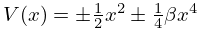
… ►where

V(x)

is the potential energy, and

x(t)

is the coordinate as a function of time

t

. … ►

22.19.5

V(x)=\pm\tfrac{1}{2}x^{2}\pm\tfrac{1}{4}\beta x^{4}

ⓘ

Symbols:: $V(x)$ : potential energy, $x(t)$ : coordinate and $\beta$ : real positive
Permalink:: http://dlmf.nist.gov/22.19.E5
Encodings:: pMML, png, TeX
See also:: Annotations for §22.19(ii), §22.19 and Ch.22

… ►

Case I: $V(x)=\frac{1}{2}x^{2}+\frac{1}{4}\beta x^{4}$

… ►

Case II: $V(x)=\frac{1}{2}x^{2}-\frac{1}{4}\beta x^{4}$

… ►

Case III: $V(x)=-\frac{1}{2}x^{2}+\frac{1}{4}\beta x^{4}$

…

26: 7.25 Software

… ►

§7.25(vi) $\mathcal{F}\left(x\right)$ , $G\left(x\right)$ , $\mathsf{U}\left(x,t\right)$ , $\mathsf{V}\left(x,t\right)$ , $x\in\mathbb{R}$

…

27: 13.1 Special Notation

… ►Other notations are:

{{}_{1}F_{1}}\left(a;b;z\right)

(§16.2(i)) and

\Phi(a;b;z)

(Humbert (1920)) for

M\left(a,b,z\right)

;

\Psi(a;b;z)

(Erdélyi et al. (1953a, §6.5)) for

U\left(a,b,z\right)

;

V(b-a,b,z)

(Olver (1997b, p. 256)) for

e^{z}U\left(a,b,-z\right)

;

\Gamma\left(1+2\mu\right)\mathscr{M}_{\kappa,\mu}

(Buchholz (1969, p. 12)) for

M_{\kappa,\mu}\left(z\right)

. …

28: 10.73 Physical Applications

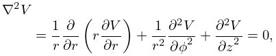
… ►Bessel functions of the first kind,

J_{n}\left(x\right)

, arise naturally in applications having cylindrical symmetry in which the physics is described either by Laplace’s equation

\nabla^{2}V=0

, or by the Helmholtz equation

(\nabla^{2}+k^{2})\psi=0

. … ►

10.73.1

\nabla^{2}V=\frac{1}{r}\frac{\partial}{\partial r}\left(r\frac{\partial V}{% \partial r}\right)+\frac{1}{r^{2}}\frac{{\partial}^{2}V}{{\partial\phi}^{2}}+% \frac{{\partial}^{2}V}{{\partial z}^{2}}=0,

ⓘ

Symbols:: $\frac{\partial\NVar{f}}{\partial\NVar{x}}$ : partial derivative of $f$ with respect to $x$ and $\,\partial\NVar{x}$ : partial differential of $x$
Permalink:: http://dlmf.nist.gov/10.73.E1
Encodings:: pMML, png, TeX
See also:: Annotations for §10.73(i), §10.73 and Ch.10

…

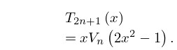
29: 18.6 Symmetry, Special Values, and Limits to Monomials

… ►

Table 18.6.1: Classical OP’s: symmetry and special values.

► ►►►►

$p_{n}(x)$	$p_{n}(-x)$	$p_{n}(1)$	$p_{2n}(0)$	$p_{2n+1}^{\prime}(0)$
…
$V_{n}\left(x\right)$	$(-1)^{n}W_{n}\left(x\right)$	$1$	$(-1)^{n}$	$(-1)^{n}(2n+2)$
$W_{n}\left(x\right)$	$(-1)^{n}V_{n}\left(x\right)$	$2n+1$	$(-1)^{n}$	$(-1)^{n}(2n+2)$
…

► …

30: 31.15 Stieltjes Polynomials

… ►There exist at most

\genfrac{(}{)}{0.0pt}{}{n+N-2}{N-2}

polynomials

V(z)

of degree not exceeding

N-2

such that for

\Phi(z)=V(z)

, (31.15.1) has a polynomial solution

w=S(z)

of degree

n

. The

V(z)

are called Van Vleck polynomials and the corresponding

S(z)

Stieltjes polynomials. … ►If

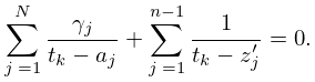
t_{k}

is a zero of the Van Vleck polynomial

V(z)

, corresponding to an

n

th degree Stieltjes polynomial

S(z)

, and

z_{1}^{\prime},z_{2}^{\prime},\dots,z_{n-1}^{\prime}

are the zeros of

S^{\prime}(z)

(the derivative of

S(z)

), then

t_{k}

is either a zero of

S^{\prime}(z)

or a solution of the equation ►

31.15.3

\sum_{j=1}^{N}\frac{\gamma_{j}}{t_{k}-a_{j}}+\sum_{j=1}^{n-1}\frac{1}{t_{k}-z_% {j}^{\prime}}=0.

ⓘ

Symbols:: $z$ : complex variable, $\gamma$ : real or complex parameter, $j$ : nonnegative integer, $n$ : nonnegative integer, $a$ : complex parameter, $N+1$ : number of singularities and $t_{k}$ : zero of $V(z)$
Permalink:: http://dlmf.nist.gov/31.15.E3
Encodings:: pMML, png, TeX
See also:: Annotations for §31.15(ii), §31.15 and Ch.31

…

���������������������������������V���ATV1819���e3y6

21—30 of 69 matching pages

21: 5.14 Multidimensional Integrals

22: 12.1 Special Notation

23: 18.7 Interrelations and Limit Relations

24: 1.18 Linear Second Order Differential Operators and Eigenfunction Expansions

25: 22.19 Physical Applications

Case I: V ⁡ ( x ) = 1 2 ⁢ x 2 + 1 4 ⁢ β ⁢ x 4

Case II: V ⁡ ( x ) = 1 2 ⁢ x 2 − 1 4 ⁢ β ⁢ x 4

Case III: V ⁡ ( x ) = − 1 2 ⁢ x 2 + 1 4 ⁢ β ⁢ x 4

26: 7.25 Software

§7.25(vi) ℱ ⁡ ( x ) , G ⁡ ( x ) , 𝖴 ⁡ ( x , t ) , 𝖵 ⁡ ( x , t ) , x ∈ ℝ

27: 13.1 Special Notation

28: 10.73 Physical Applications

29: 18.6 Symmetry, Special Values, and Limits to Monomials

30: 31.15 Stieltjes Polynomials

��V��ATV1819��e3y6

Case I: $V(x)=\frac{1}{2}x^{2}+\frac{1}{4}\beta x^{4}$

Case II: $V(x)=\frac{1}{2}x^{2}-\frac{1}{4}\beta x^{4}$

Case III: $V(x)=-\frac{1}{2}x^{2}+\frac{1}{4}\beta x^{4}$

§7.25(vi) $\mathcal{F}\left(x\right)$ , $G\left(x\right)$ , $\mathsf{U}\left(x,t\right)$ , $\mathsf{V}\left(x,t\right)$ , $x\in\mathbb{R}$