������������������������������/������������/������������������CXFK69���epWz5VZ
The term"CXFK69" was not found.
(0.038 seconds)
1—10 of 676 matching pages
1: 4.17 Special Values and Limits
2: 24.2 Definitions and Generating Functions
3: 12.7 Relations to Other Functions
…
►
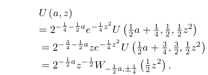
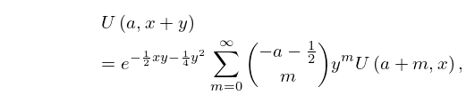
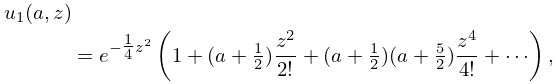
12.7.8
…
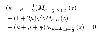
►For these, the corresponding results for with , , , , , and the corresponding results for with , , , , , , , see Miller (1955, pp. 42–43 and 77–79).
…
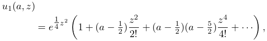
►
12.7.12
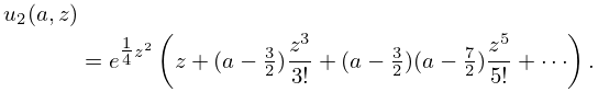
►
12.7.13
…
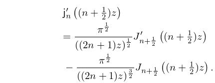
►
12.7.14
…
4: 26.3 Lattice Paths: Binomial Coefficients
…
►
is the number of ways of choosing objects from a collection of distinct objects without regard to order.
is the number of lattice paths from to .
…The number of lattice paths from to , , that stay on or above the line is
…
►For numerical values of and see Tables 26.3.1 and 26.3.2.
►
…
5: 13.15 Recurrence Relations and Derivatives
6: 12.13 Sums
7: 12.4 Power-Series Expansions
8: 10.57 Uniform Asymptotic Expansions for Large Order
…
►Asymptotic expansions for , , , , , and as that are uniform with respect to can be obtained from the results given in §§10.20 and 10.41 by use of the definitions (10.47.3)–(10.47.7) and (10.47.9).
Subsequently, for the connection formula (10.47.11) is available.
►For the corresponding expansion for use
►
10.57.1
…
