欢乐斗地主改名字【亚博官方qee9.com】3d福彩缩水17o
(0.004 seconds)
11—20 of 733 matching pages
11: Bibliography Z
…
►
On the Computation of Zeros of Bessel and Bessel-related Functions.
In Proceedings of the Sixth International Colloquium on
Differential Equations (Plovdiv, Bulgaria, 1995), D. Bainov (Ed.),
Utrecht, pp. 409–416.
…
►
Remark on “Algorithm 916: computing the Faddeyeva and Voigt functions”: efficiency improvements and Fortran translation.
ACM Trans. Math. Softw. 42 (3), pp. 26:1–26:9.
…
►
Weighted derangements and the linearization coefficients of orthogonal Sheffer polynomials.
Proc. London Math. Soc. (3) 65 (1), pp. 1–22.
…
►
Mathieu functions for purely imaginary parameters.
J. Comput. Appl. Math. 236 (17), pp. 4513–4524.
…
►
Fast evaluation of elementary mathematical functions with correctly rounded last bit.
ACM Trans. Math. Software 17 (3), pp. 410–423.
…
12: 34.8 Approximations for Large Parameters
§34.8 Approximations for Large Parameters
►For large values of the parameters in the , , and symbols, different asymptotic forms are obtained depending on which parameters are large. … ►and the symbol denotes a quantity that tends to zero as the parameters tend to infinity, as in §2.1(i). … ►Uniform approximations in terms of Airy functions for the and symbols are given in Schulten and Gordon (1975b). For approximations for the , , and symbols with error bounds see Flude (1998), Chen et al. (1999), and Watson (1999): these references also cite earlier work.13: 30.16 Methods of Computation
…
►For sufficiently large, construct the tridiagonal matrix with nonzero elements
…and real eigenvalues , , , , arranged in ascending order of magnitude.
…
►Let be the matrix given by (30.16.1) if is even, or by (30.16.6) if is odd.
Form the eigenvector of associated with the eigenvalue , , normalized according to
…
►The coefficients calculated in §30.16(ii) can be used to compute , from (30.11.3) as well as the connection coefficients from (30.11.10) and (30.11.11).
…
14: Bibliography S
…
►
Numerical evaluation of integrals of the form and the tabulation of the function
.
Quart. J. Mech. Appl. Math. 3 (1), pp. 107–112.
…
►
Asymptotic solutions of nonlinear evolution equations and a Painlevé transcendent.
Phys. D 3 (1-2), pp. 165–184.
…
►
Inequalities involving cylindrical functions of nearly equal argument and order.
Proc. Amer. Math. Soc. 5 (3), pp. 337–344.
…
►
Some comments on Fourier analysis, uncertainty and modeling.
SIAM Rev. 25 (3), pp. 379–393.
…
►
On the relative extrema of ultraspherical polynomials.
Boll. Un. Mat. Ital. (3) 5, pp. 125–127.
…
15: 34.14 Tables
§34.14 Tables
►Tables of exact values of the squares of the and symbols in which all parameters are are given in Rotenberg et al. (1959), together with a bibliography of earlier tables of , and symbols on pp. … ►Tables of and symbols in which all parameters are are given in Appel (1968) to 6D. …Other tabulations for symbols are listed on pp. … ►In Varshalovich et al. (1988) algebraic expressions for the Clebsch–Gordan coefficients with all parameters and numerical values for all parameters are given on pp. …16: 9.13 Generalized Airy Functions
…
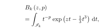
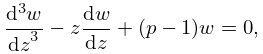
►where For real variables the solutions of (9.13.13) are denoted by , when is even, and by , when is odd.
…
►
9.13.27
, ,
…
►The integration paths , , , are depicted in Figure 9.13.1.
, , are depicted in Figure 9.13.2.
…
►
9.13.31
…
17: 28.8 Asymptotic Expansions for Large
…
►
…
28.8.1
►For recurrence relations for the coefficients in these expansions see Frenkel and Portugal (2001, §3).
…
►
28.8.2
…
►Also let and (§18.3).
…
►
18: 32.11 Asymptotic Approximations for Real Variables
…
►and and are constants.
…
►
(c)
…
►Connection formulas for and are given by
…
►Connection formulas for and are given by
…
►In terms of the parameter that is used in these figures .
…
If , then changes sign once, from positive to negative, as passes from to .
19: 25.16 Mathematical Applications
…
►
►
…
►
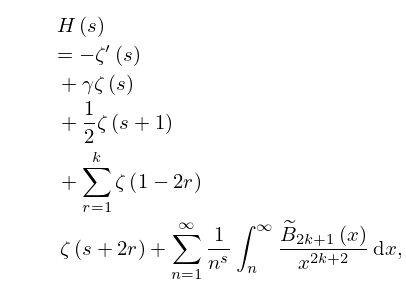
has a simple pole with residue () at each odd negative integer , .
…
►
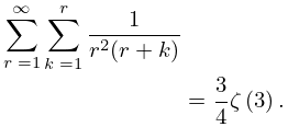
25.16.6
…
►
25.16.15
…
