办假的科罗拉多学院文凭毕业证【somewhat微aptao168】bigrf
The term"aptao168" was not found.Possible alternative term: "caption".
(0.002 seconds)
1—10 of 28 matching pages
1: Software Index
…
►
►
…
►
Open Source Collections and Systems.
…
| Open Source | With Book | Commercial | |||||||||||||||||||||||
| … | |||||||||||||||||||||||||
| 19.39(iv) , , , | ✓ | ✓ | ✓ | ✓ | a | ✓ | ✓ | ✓ | ✓ | Derive | |||||||||||||||
| … | |||||||||||||||||||||||||
These are collections of software (e.g. libraries) or interactive systems of a somewhat broad scope. Contents may be adapted from research software or may be contributed by project participants who donate their services to the project. The software is made freely available to the public, typically in source code form. While formal support of the collection may not be provided by its developers, within active projects there is often a core group who donate time to consider bug reports and make updates to the collection.
2: 19.21 Connection Formulas
…
►
19.21.1
.
…
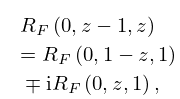
►The complete cases of and have connection formulas resulting from those for the Gauss hypergeometric function (Erdélyi et al. (1953a, §2.9)).
…
►
19.21.4
…
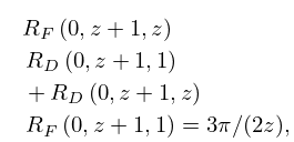
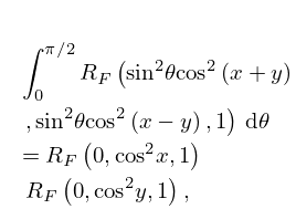
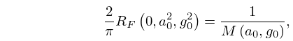
►The complete case of can be expressed in terms of and :
…
►Because is completely symmetric, can be permuted on the right-hand side of (19.21.10) so that if the variables are real, thereby avoiding cancellations when is calculated from and (see §19.36(i)).
…
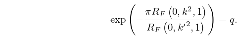
3: 19.32 Conformal Map onto a Rectangle
4: 20.9 Relations to Other Functions
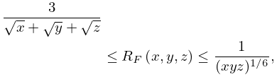
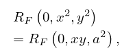
5: 19.24 Inequalities
…
►For , , and , the complete cases of and satisfy
►
…
►
…
19.24.10
…
►Other inequalities for are given in Carlson (1970).
…
►
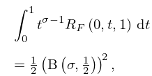
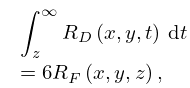
6: 19.28 Integrals of Elliptic Integrals
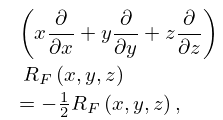
7: 19.18 Derivatives and Differential Equations
…
►
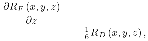
19.18.1
►
19.18.2
…
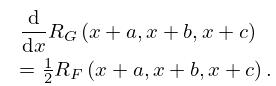
►
19.18.6
…
►
19.18.9
…
►The next four differential equations apply to the complete case of and in the form (see (19.16.20) and (19.16.23)).
…
8: 19.22 Quadratic Transformations
9: 19.36 Methods of Computation
…
►For the polynomial of degree 7, for example, is
…
►All cases of , , , and are computed by essentially the same procedure (after transforming Cauchy principal values by means of (19.20.14) and (19.2.20)).
…Because of cancellations in (19.26.21) it is advisable to compute from and by (19.21.10) or else to use §19.36(ii).
…
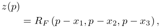
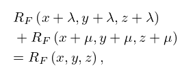
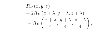
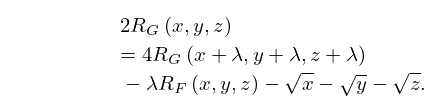
►We compute by setting , , and .
…
►Similarly, §19.26(ii) eases the computation of functions such as when () is small compared with .
…
