%E7%AB%9E%E5%BD%A9%E8%B6%B3%E7%90%83%E8%BF%87%E5%85%B3%E6%96%B9%E5%BC%8F3%C3%971%E3%80%90%E4%BA%9A%E5%8D%9A%E5%AE%98%E6%96%B9qee9.com%E3%80%91%E7%94%B5%E8%84%91%E6%AC%A2%E4%B9%90%E6%96%97%E5%9C%B0%E4%B8%BB%E5%9C%A8%E5%93%AA%E9%87%8CNuq7IN

SearchAdvancedHelp

(0.024 seconds)

21—30 of 552 matching pages

21: 19.9 Inequalities

… ►

$1\le E\left(k\right)\le \pi /2.$

… ►

19.9.3

ⓘ

Symbols:

$K\left(k\right)$: Legendre’s complete elliptic integral of the first kind, $\ln z$: principal branch of logarithm function, $k$: real or complex modulus and $k^{\prime }$: complementary modulus

Referenced by:

§19.9(i), §19.9(i)

Permalink:

http://dlmf.nist.gov/19.9.E3

Encodings:

pMML, png, TeX

See also:

Annotations for §19.9(i), §19.9 and Ch.19

… ►Further inequalities for $K\left(k\right)$ and $E\left(k\right)$ can be found in Alzer and Qiu (2004), Anderson et al. (1992a, b, 1997), and Qiu and Vamanamurthy (1996). … ►

19.9.9 $$L(a,b)=4aE\left(k\right),$$ $k^2=1-(b^2/a^2)$, $a>b$.

ⓘ

Symbols:

$E\left(k\right)$: Legendre’s complete elliptic integral of the second kind, $k$: real or complex modulus and $L(a,b)$: perimeter

Referenced by:

§19.9(i)

Permalink:

http://dlmf.nist.gov/19.9.E9

Encodings:

pMML, png, TeX

See also:

Annotations for §19.9(i), §19.9 and Ch.19

… ►Inequalities for both $F(\varphi ,k)$ and $E(\varphi ,k)$ involving inverse circular or inverse hyperbolic functions are given in Carlson (1961b, §4). …

22: 8.4 Special Values

… ►For $E_n\left(z\right)$ see §8.19(i). … ►

8.4.4 $$\mathrm{\Gamma }(0,z)={\int }_z^{\mathrm{\infty }}{t}^{-1}{\mathrm{e}}^{-t}dt=E_1\left(z\right),$$

ⓘ

Symbols:

$dx$: differential of $x$ , $\mathrm{e}$: base of natural logarithm, $E_1\left(z\right)$: exponential integral, $\mathrm{\Gamma }(a,z)$: incomplete gamma function, $\int$: integral and $z$: complex variable

A&S Ref:

6.5.15

Permalink:

http://dlmf.nist.gov/8.4.E4

Encodings:

pMML, png, TeX

See also:

Annotations for §8.4 and Ch.8

… ►

8.4.13 $$\mathrm{\Gamma }(1-n,z)=z^{1-n}{E}_n\left(z\right),$$

ⓘ

Symbols:

$E_p\left(z\right)$: generalized exponential integral, $\mathrm{\Gamma }(a,z)$: incomplete gamma function, $z$: complex variable and $n$: nonnegative integer

Referenced by:

§8.19(iv)

Permalink:

http://dlmf.nist.gov/8.4.E13

Encodings:

pMML, png, TeX

See also:

Annotations for §8.4 and Ch.8

… ►

8.4.15 $$\mathrm{\Gamma }(-n,z)=\frac{{(-1)}^n}{n!}\left(E_1\left(z\right)-{\mathrm{e}}^{-z}\sum _{k=0}^{n-1}\frac{{(-1)}^{k}k!}{z^{k+1}}\right)=\frac{{(-1)}^n}{n!}\left(\psi \left(n+1\right)-\ln z\right)-z^{-n}\sum _{\begin{array}{c}k=0\\ k\ne n\end{array}}^{\mathrm{\infty }}\frac{{(-z)}^k}{k!(k-n)}.$$

ⓘ

Symbols:

$\psi \left(z\right)$: psi (or digamma) function, $\mathrm{e}$: base of natural logarithm, $E_1\left(z\right)$: exponential integral, $!$: factorial (as in $n!$), $\mathrm{\Gamma }(a,z)$: incomplete gamma function, $\ln z$: principal branch of logarithm function, $z$: complex variable, $k$: nonnegative integer and $n$: nonnegative integer

A&S Ref:

6.5.19

Referenced by:

§8.19(iii), §8.19(iv), §8.4

Permalink:

http://dlmf.nist.gov/8.4.E15

Encodings:

pMML, png, TeX

See also:

Annotations for §8.4 and Ch.8

23: Software Index

… ► ►►►►►►►

	Open Source													With Book						Commercial
…
8.28(vii) $E_p\left(z\right)$, $z,p\in ℂ$	✓											✓	✓								✓	✓	✓
9 Airy and Related Functions
…
11.16(v) ${𝐉}_{\nu }\left(z\right)$, ${𝐄}_{\nu }\left(z\right)$, ${𝐀}_{\nu }\left(z\right)$												a	✓				✓				✓	✓	a
…
24.21(ii) $B_n$, $B_n\left(x\right)$, $E_n$, $E_n\left(x\right)$	✓	✓						✓		✓		a	✓	✓			✓		✓		✓	✓	✓		Derive, MuPAD
…
34 3j, 6j, 9j Symbols
…

…

24: 16.7 Relations to Other Functions

… ►For $\mathit{3}j$, $\mathit{6}j$, $\mathit{9}j$ symbols see Chapter 34. …

25: 34.8 Approximations for Large Parameters

§34.8 Approximations for Large Parameters

►For large values of the parameters in the $\mathit{3}j$, $\mathit{6}j$, and $\mathit{9}j$ symbols, different asymptotic forms are obtained depending on which parameters are large. … ►For approximations for the $\mathit{3}j$, $\mathit{6}j$, and $\mathit{9}j$ symbols with error bounds see Flude (1998), Chen et al. (1999), and Watson (1999): these references also cite earlier work.

26: 19.5 Maclaurin and Related Expansions

… ►

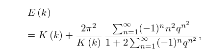
19.5.6 $$q=\lambda +2{\lambda }^5+15{\lambda }^9+150{\lambda }^{13}+1707{\lambda }^{17}+\mathrm{\cdots },$$ $0\le k\le 1$,

ⓘ

Symbols:

$q$: nome and $k$: real or complex modulus

Referenced by:

§19.5, §19.5

Permalink:

http://dlmf.nist.gov/19.5.E6

Encodings:

pMML, png, TeX

See also:

Annotations for §19.5 and Ch.19

… ►Coefficients of terms up to ${\lambda }^{49}$ are given in Lee (1990), along with tables of fractional errors in $K\left(k\right)$ and $E\left(k\right)$, $0.1\le k^2\le 0.9999$, obtained by using 12 different truncations of (19.5.6) in (19.5.8) and (19.5.9). … ►

19.5.9 $$E\left(k\right)=K\left(k\right)+\frac{2{\pi }^2}{K\left(k\right)}\frac{{\sum }_{n=1}^{\mathrm{\infty }}{(-1)}^n{n}^2{q}^{n^2}}{1+2{\sum }_{n=1}^{\mathrm{\infty }}{(-1)}^n{q}^{n^2}},$$ .

ⓘ

Symbols:

$\pi$: the ratio of the circumference of a circle to its diameter, $K\left(k\right)$: Legendre’s complete elliptic integral of the first kind, $E\left(k\right)$: Legendre’s complete elliptic integral of the second kind, $q$: nome, $n$: nonnegative integer and $k$: real or complex modulus

Referenced by:

§19.5, §19.5

Permalink:

http://dlmf.nist.gov/19.5.E9

Encodings:

pMML, png, TeX

See also:

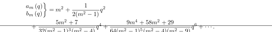
Annotations for §19.5 and Ch.19

… ►Series expansions of $F(\varphi ,k)$ and $E(\varphi ,k)$ are surveyed and improved in Van de Vel (1969), and the case of $F(\varphi ,k)$ is summarized in Gautschi (1975, §1.3.2). For series expansions of $\mathrm{\Pi }(\varphi ,{\alpha }^2,k)$ when see Erdélyi et al. (1953b, §13.6(9)). …

27: 3.5 Quadrature

… ►If $f\in C^{2m+2}[a,b]$, then the remainder $E_n(f)$ in (3.5.2) can be expanded in the form … ►About $2^9=512$ function evaluations are needed. … ►with weight function $w(x)$, is one for which $E_n(f)=0$ whenever $f$ is a polynomial of degree $\le n-1$. The nodes $x_1,x_2,\mathrm{\dots },x_n$ are prescribed, and the weights $w_k$ and error term $E_n(f)$ are found by integrating the product of the Lagrange interpolation polynomial of degree $n-1$ and $w(x)$. … ►where $E_n(f)=0$ if $f(\zeta )$ is a polynomial of degree $\le 2n-1$ in $1/\zeta$. …

28: 28.6 Expansions for Small $q$

… ►Leading terms of the of the power series for $m=7,8,9,\mathrm{\dots }$ are: ►

28.6.14 $$\begin{array}{c}{a}_m\left(q\right)\\ b_m\left(q\right)\end{array}\}=m^2+\frac{1}{2(m^2-1)}{q}^2+\frac{5m^2+7}{32{(m^2-1)}^3(m^2-4)}{q}^4+\frac{9m^4+58m^2+29}{64{(m^2-1)}^5(m^2-4)(m^2-9)}{q}^6+\mathrm{\cdots }.$$

ⓘ

Symbols:

$a_n\left(q\right)$: eigenvalues of Mathieu equation, $b_n\left(q\right)$: eigenvalues of Mathieu equation, $m$: integer and $q=h^2$: parameter

A&S Ref:

20.2.26

Referenced by:

§28.6(i), §28.6(i), Erratum (V1.1.10) for Sections 28.6(i), 28.6(ii), 28.8(i), 28.8(ii)

Permalink:

http://dlmf.nist.gov/28.6.E14

Encodings:

pMML, png, TeX

See also:

Annotations for §28.6(i), §28.6 and Ch.28

… ►Numerical values of the radii of convergence ${\rho }_n^{(j)}$ of the power series (28.6.1)–(28.6.14) for $n=0,1,\mathrm{\dots },9$ are given in Table 28.6.1. … ►where $k$ is the unique root of the equation $2E\left(k\right)=K\left(k\right)$ in the interval $(0,1)$, and $k^{\prime }=\sqrt{1-k^2}$. For $E\left(k\right)$ and $K\left(k\right)$ see §19.2(ii). …

29: 3.6 Linear Difference Equations

… ►The Weber function ${𝐄}_n\left(1\right)$ satisfies …Thus the asymptotic behavior of the particular solution ${𝐄}_n\left(1\right)$ is intermediate to those of the complementary functions $J_n\left(1\right)$ and $Y_n\left(1\right)$; moreover, the conditions for Olver’s algorithm are satisfied. We apply the algorithm to compute ${𝐄}_n\left(1\right)$ to 8S for the range $n=1,2,\mathrm{\dots },10$, beginning with the value ${𝐄}_0\left(1\right)=-\mathrm{0.56865\hspace{0.33em}\hspace{0.17em}663}$ obtained from the Maclaurin series expansion (§11.10(iii)). … ►The values of $w_n$ for $n=1,2,\mathrm{\dots },10$ are the wanted values of ${𝐄}_n\left(1\right)$. (It should be observed that for $n>10$, however, the $w_n$ are progressively poorer approximations to ${𝐄}_n\left(1\right)$: the underlined digits are in error.) …

30: 24.12 Zeros

… ►For the interval denote the zeros of $E_n\left(x\right)$ by $y_j^{(n)}$, $j=1,2,\mathrm{\dots }$, with … ►

24.12.10 $n=5,9,13,\mathrm{\dots }$,

ⓘ

Symbols:

$\pi$: the ratio of the circumference of a circle to its diameter, $!$: factorial (as in $n!$), $n$: integer and $y_j^{(n)}$: zeros

Permalink:

http://dlmf.nist.gov/24.12.E10

Encodings:

pMML, png, TeX

See also:

Annotations for §24.12(ii), §24.12 and Ch.24

… ►The only polynomial $E_n\left(x\right)$ with multiple zeros is $E_5\left(x\right)=(x-\frac{1}{2}){(x^2-x-1)}^2$.