%E6%A2%AD%E5%93%88%E6%B8%B8%E6%88%8F%E5%A4%A7%E5%8E%85,%E7%BD%91%E4%B8%8A%E6%A2%AD%E5%93%88%E6%B8%B8%E6%88%8F%E8%A7%84%E5%88%99,%E3%80%90%E5%A4%8D%E5%88%B6%E6%89%93%E5%BC%80%E7%BD%91%E5%9D%80%EF%BC%9A33kk55.com%E3%80%91%E6%AD%A3%E8%A7%84%E5%8D%9A%E5%BD%A9%E5%B9%B3%E5%8F%B0,%E5%9C%A8%E7%BA%BF%E8%B5%8C%E5%8D%9A%E5%B9%B3%E5%8F%B0,%E6%A2%AD%E5%93%88%E6%B8%B8%E6%88%8F%E7%8E%A9%E6%B3%95%E4%BB%8B%E7%BB%8D,%E7%9C%9F%E4%BA%BA%E6%A2%AD%E5%93%88%E6%B8%B8%E6%88%8F%E8%A7%84%E5%88%99,%E7%BD%91%E4%B8%8A%E7%9C%9F%E4%BA%BA%E6%A3%8B%E7%89%8C%E6%B8%B8%E6%88%8F%E5%B9%B3%E5%8F%B0,%E7%9C%9F%E4%BA%BA%E5%8D%9A%E5%BD%A9%E6%B8%B8%E6%88%8F%E5%B9%B3%E5%8F%B0%E7%BD%91%E5%9D%80YCBNyMNNVhsBhNMy

SearchAdvancedHelp

(0.081 seconds)

11—20 of 673 matching pages

11: 19.36 Methods of Computation

… ►For $R_F$ the polynomial of degree 7, for example, is … ►All cases of $R_F$, $R_C$, $R_J$, and $R_D$ are computed by essentially the same procedure (after transforming Cauchy principal values by means of (19.20.14) and (19.2.20)). … ►The incomplete integrals $R_F(x,y,z)$ and $R_G(x,y,z)$ can be computed by successive transformations in which two of the three variables converge quadratically to a common value and the integrals reduce to $R_C$, accompanied by two quadratically convergent series in the case of $R_G$; compare Carlson (1965, §§5,6). … ► $F(\varphi ,k)$ can be evaluated by using (19.25.5). …A summary for $F(\varphi ,k)$ is given in Gautschi (1975, §3). …

12: 9.4 Maclaurin Series

… ►

9.4.1 $$\mathrm{Ai}\left(z\right)=\mathrm{Ai}\left(0\right)\left(1+\frac{1}{3!}{z}^3+\frac{1\cdot 4}{6!}{z}^6+\frac{1\cdot 4\cdot 7}{9!}{z}^9+\mathrm{\cdots }\right)+{\mathrm{Ai}}^{\prime }\left(0\right)\left(z+\frac{2}{4!}{z}^4+\frac{2\cdot 5}{7!}{z}^7+\frac{2\cdot 5\cdot 8}{10!}{z}^{10}+\mathrm{\cdots }\right),$$

ⓘ

Symbols:

$\mathrm{Ai}\left(z\right)$: Airy function, $!$: factorial (as in $n!$) and $z$: complex variable

Source:

Olver (1997b, p. 54)

A&S Ref:

10.4.2 (with 10.4.4 and 10.4.5)

Permalink:

http://dlmf.nist.gov/9.4.E1

Encodings:

pMML, png, TeX

See also:

Annotations for §9.4 and Ch.9

►

9.4.2 $${\mathrm{Ai}}^{\prime }\left(z\right)={\mathrm{Ai}}^{\prime }\left(0\right)\left(1+\frac{2}{3!}{z}^3+\frac{2\cdot 5}{6!}{z}^6+\frac{2\cdot 5\cdot 8}{9!}{z}^9+\mathrm{\cdots }\right)+\mathrm{Ai}\left(0\right)\left(\frac{1}{2!}{z}^2+\frac{1\cdot 4}{5!}{z}^5+\frac{1\cdot 4\cdot 7}{8!}{z}^8+\mathrm{\cdots }\right),$$

ⓘ

Symbols:

$\mathrm{Ai}\left(z\right)$: Airy function, $!$: factorial (as in $n!$) and $z$: complex variable

Proof sketch:

Use methods of Olver (1997b, p. 54).

Permalink:

http://dlmf.nist.gov/9.4.E2

Encodings:

pMML, png, TeX

See also:

Annotations for §9.4 and Ch.9

►

9.4.3 $$\mathrm{Bi}\left(z\right)=\mathrm{Bi}\left(0\right)\left(1+\frac{1}{3!}{z}^3+\frac{1\cdot 4}{6!}{z}^6+\frac{1\cdot 4\cdot 7}{9!}{z}^9+\mathrm{\cdots }\right)+{\mathrm{Bi}}^{\prime }\left(0\right)\left(z+\frac{2}{4!}{z}^4+\frac{2\cdot 5}{7!}{z}^7+\frac{2\cdot 5\cdot 8}{10!}{z}^{10}+\mathrm{\cdots }\right),$$

ⓘ

Symbols:

$\mathrm{Bi}\left(z\right)$: Airy function, $!$: factorial (as in $n!$) and $z$: complex variable

Proof sketch:

Use methods of Olver (1997b, p. 54).

A&S Ref:

10.4.3 (with 10.4.4 and 10.4.5)

Referenced by:

(9.12.15)

Permalink:

http://dlmf.nist.gov/9.4.E3

Encodings:

pMML, png, TeX

See also:

Annotations for §9.4 and Ch.9

►

9.4.4 $${\mathrm{Bi}}^{\prime }\left(z\right)={\mathrm{Bi}}^{\prime }\left(0\right)\left(1+\frac{2}{3!}{z}^3+\frac{2\cdot 5}{6!}{z}^6+\frac{2\cdot 5\cdot 8}{9!}{z}^9+\mathrm{\cdots }\right)+\mathrm{Bi}\left(0\right)\left(\frac{1}{2!}{z}^2+\frac{1\cdot 4}{5!}{z}^5+\frac{1\cdot 4\cdot 7}{8!}{z}^8+\mathrm{\cdots }\right).$$

ⓘ

Symbols:

$\mathrm{Bi}\left(z\right)$: Airy function, $!$: factorial (as in $n!$) and $z$: complex variable

Proof sketch:

Use methods of Olver (1997b, p. 54).

Permalink:

http://dlmf.nist.gov/9.4.E4

Encodings:

pMML, png, TeX

See also:

Annotations for §9.4 and Ch.9

13: 18.8 Differential Equations

… ►

Table 18.8.1: Classical OP’s: differential equations $A(x)f^{\prime \prime }(x)+B(x)f^{\prime }(x)+C(x)f(x)+{\lambda }_{n}f(x)=0$.

► ►►►►►

#	$f(x)$	$A(x)$	$B(x)$	$C(x)$	${\lambda }_n$
…
4	$C_n^{(\lambda )}\left(x\right)$	$1-x^2$	$-(2\lambda +1)x$	$0$	$n(n+2\lambda )$
…
8	$L_n^{(\alpha )}\left(x\right)$	$x$	$\alpha +1-x$	$0$	$n$
9	${\mathrm{e}}^{-\frac{1}{2}{x}^2}{x}^{\alpha +\frac{1}{2}}{L}_n^{(\alpha )}\left(x^2\right)$	$1$	$0$	$-x^2+(\frac{1}{4}-{\alpha }^2)x^{-2}$	$4n+2\alpha +2$
…

►

…

14: 3.3 Interpolation

… ►If $f$ is analytic in a simply-connected domain $D$ (§1.13(i)), then for $z\in D$, …where $C$ is a simple closed contour in $D$ described in the positive rotational sense and enclosing the points $z,z_1,z_2,\mathrm{\dots },z_n$. … ►where ${\omega }_{n+1}(\zeta )$ is given by (3.3.3), and $C$ is a simple closed contour in $D$ described in the positive rotational sense and enclosing $z_0,z_1,\mathrm{\dots },z_n$. … ►By using this approximation to $x$ as a new point, $x_3=x$, and evaluating $\left[f_0,f_1,f_2,f_3\right]x=\mathrm{1.12388\hspace{0.33em}6190}$, we find that $x=-\mathrm{2.33810\hspace{0.33em}7409}$, with 9 correct digits. … ►Then by using $x_3$ in Newton’s interpolation formula, evaluating $\left[x_0,x_1,x_2,x_3\right]f=-\mathrm{0.26608\hspace{0.33em}28233}$ and recomputing $f^{\prime }(x)$, another application of Newton’s rule with starting value $x_3$ gives the approximation $x=\mathrm{2.33810\hspace{0.33em}7373}$, with 8 correct digits. …

15: 18.5 Explicit Representations

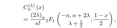
… ►In (18.5.4_5) see §26.11 for the Fibonacci numbers $F_n$. … ►In this equation $w(x)$ is as in Table 18.3.1, (reproduced in Table 18.5.1), and $F(x)$, ${\kappa }_n$ are as in Table 18.5.1. … ►For the definitions of ${}_2{}^{}F_1^{}$, ${}_1{}^{}F_1^{}$, and ${}_2{}^{}F_0^{}$ see §16.2. … ►

18.5.9 $$C_n^{(\lambda )}\left(x\right)=\frac{{\left(2\lambda \right)}_n}{n!}{}_2{}^{}F_1^{}(\genfrac{}{}{0pt}{}{-n,n+2\lambda }{\lambda +\frac{1}{2}};\frac{1-x}{2}),$$

ⓘ

Symbols:

${}_2{}^{}F_1^{}(a,b;c;z)$: $=F(a,b;c;z)$ notation for Gauss’ hypergeometric function, ${\left(a\right)}_n$: Pochhammer’s symbol (or shifted factorial), $!$: factorial (as in $n!$), $C_n^{(\lambda )}\left(x\right)$: ultraspherical (or Gegenbauer) polynomial, $n$: nonnegative integer and $x$: real variable

A&S Ref:

22.5.46

Referenced by:

§18.5(iii), §18.6(i)

Permalink:

http://dlmf.nist.gov/18.5.E9

Encodings:

pMML, png, TeX

See also:

Annotations for §18.5(iii), §18.5(iii), §18.5 and Ch.18

… ►Similarly in the cases of the ultraspherical polynomials $C_n^{(\lambda )}\left(x\right)$ and the Laguerre polynomials $L_n^{(\alpha )}\left(x\right)$ we assume that $\lambda >-\frac{1}{2},\lambda \ne 0$, and $\alpha >-1$, unless stated otherwise. …

16: Bibliography T

… ►

The universal Askey-Wilson algebra and DAHA of type $(C_1^{\vee },C_1)$ . SIGMA 9, pp. Paper 047, 40 pp..

ⓘ

External Links:

ISSN 1815-0659, Link, MathReview (Renato Álvarez-Nodarse), ZentralBlatt

Referenced by:

§18.38(iii).

Encodings:

BibTeX

… ►

Algorithm 926: incomplete gamma functions with negative arguments. ACM Trans. Math. Software 39 (2), pp. Art. 14, 9.

ⓘ

External Links:

ISSN 0098-3500, Document, FullText, MathReview Entry, ZentralBlatt

Referenced by:

7th item, §8.28(ii).

Encodings:

BibTeX

… ►

Angular Momentum: An Illustrated Guide to Rotational Symmetries for Physical Systems. A Wiley-Interscience Publication, John Wiley & Sons Inc., New York.

ⓘ

Notes:

With 1 Macintosh floppy disk (3.5 inch; DD). Programs for the calculation of $3j,6j,9j$ symbols are included.

External Links:

ISBN 0-471-55264-X, MathReview (J. F. Cornwell), ZentralBlatt

Referenced by:

§34.3(vii).

Encodings:

BibTeX

… ►

Rational Chebyshev approximation for the Fermi-Dirac integral $F_{-3/2}(x)$ . Solid–State Electronics 41 (5), pp. 771–773.

ⓘ

External Links:

Document

Referenced by:

§25.21(vii).

Encodings:

BibTeX

… ►

Theory of the Fresnel integral. USSR Comput. Math. and Math. Phys. 9 (4), pp. 271–279.

ⓘ

Notes:

Translation of the paper in Zh. Vychisl. Mat. Mat. Fiz., Vol. 9, No. 4, 938-944, 1969

External Links:

Document, ZentralBlatt

Referenced by:

§7.13(iv).

Encodings:

BibTeX

17: 15.3 Graphics

… ►

►►

Figure 15.3.1: $F(\frac{4}{3},\frac{9}{16};\frac{14}{5};x),-100\le x\le 1$. Magnify

►

►►

Figure 15.3.2: $F(5,-10;1;x),-0.023\le x\le 1$. Magnify

►

►►

Figure 15.3.3: $F(1,-10;10;x),-3\le x\le 1$. Magnify

►

►►

Figure 15.3.4: $F(5,10;1;x),-1\le x\le 0.022$. Magnify

… ►

►

►

Figure 15.3.5: $F(\frac{4}{3},\frac{9}{16};\frac{14}{5};x+\mathrm{i}y),0\le x\le 2,-0.5\le y\le 0.5$. … Magnify 3D Help

…

18: 14.33 Tables

… ►

Abramowitz and Stegun (1964, Chapter 8) tabulates ${𝖯}_n\left(x\right)$ for $n=0(1)3,9,10$, $x=0(.01)1$, 5–8D; ${𝖯}_n^{\prime }\left(x\right)$ for $n=1(1)4,9,10$, $x=0(.01)1$, 5–7D; ${𝖰}_n\left(x\right)$ and ${𝖰}_n^{\prime }\left(x\right)$ for $n=0(1)3,9,10$, $x=0(.01)1$, 6–8D; $P_n\left(x\right)$ and $P_n^{\prime }\left(x\right)$ for $n=0(1)5,9,10$, $x=1(.2)10$, 6S; $Q_n\left(x\right)$ and $Q_n^{\prime }\left(x\right)$ for $n=0(1)3,9,10$, $x=1(.2)10$, 6S. (Here primes denote derivatives with respect to $x$.)

►

Zhang and Jin (1996, Chapter 4) tabulates ${𝖯}_n\left(x\right)$ for $n=2(1)5,10$, $x=0(.1)1$, 7D; ${𝖯}_n\left(\cos \theta \right)$ for $n=1(1)4,10$, $\theta =0(5^{\circ }){90}^{\circ }$, 8D; ${𝖰}_n\left(x\right)$ for $n=0(1)2,10$, $x=0(.1)0.9$, 8S; ${𝖰}_n\left(\cos \theta \right)$ for $n=0(1)3,10$, $\theta =0(5^{\circ }){90}^{\circ }$, 8D; ${𝖯}_n^m\left(x\right)$ for $m=1(1)4$, $n-m=0(1)2$, $n=10$, $x=0,0.5$, 8S; ${𝖰}_n^m\left(x\right)$ for $m=1(1)4$, $n=0(1)2,10$, 8S; ${𝖯}_{\nu }^m\left(\cos \theta \right)$ for $m=0(1)3$, $\nu =0(.25)5$, $\theta =0({15}^{\circ }){90}^{\circ }$, 5D; $P_n\left(x\right)$ for $n=2(1)5,10$, $x=1(1)10$, 7S; $Q_n\left(x\right)$ for $n=0(1)2,10$, $x=2(1)10$, 8S. Corresponding values of the derivative of each function are also included, as are 6D values of the first 5 $\nu$-zeros of ${𝖯}_{\nu }^m\left(\cos \theta \right)$ and of its derivative for $m=0(1)4$, $\theta ={10}^{\circ },{30}^{\circ },{150}^{\circ }$.

►

Belousov (1962) tabulates ${𝖯}_n^m\left(\cos \theta \right)$ (normalized) for $m=0(1)36$, $n-m=0(1)56$, $\theta =0({2.5}^{\circ }){90}^{\circ }$, 6D.

…

19: Bibliography K

… ►

A proof of the $q$-Macdonald-Morris conjecture for $B{C}_n$ . Mem. Amer. Math. Soc. 108 (516), pp. vi+80.

ⓘ

External Links:

ISSN 0065-9266, MathReview (Eric M. Opdam), ZentralBlatt

Referenced by:

§17.14.

Encodings:

BibTeX

… ►

Determinant structure of the rational solutions for the Painlevé II equation. J. Math. Phys. 37 (9), pp. 4693–4704.

ⓘ

External Links:

ISSN 0022-2488, Document, MathReview (Andrei A. Kapaev), ZentralBlatt

Referenced by:

§32.8(ii).

Encodings:

BibTeX

… ►

Poly-Bernoulli numbers. J. Théor. Nombres Bordeaux 9 (1), pp. 221–228.

ⓘ

External Links:

ISSN 1246-7405, PostScript, MathReview (L. Skula), ZentralBlatt

Referenced by:

§24.16(iii).

Encodings:

BibTeX

… ►

Overview of some new results concerning the theory and applications of the Rayleigh special function. Comput. Math. Math. Phys. 48 (9), pp. 1454–1507.

ⓘ

External Links:

ISSN 0965-5425, Document, FullText

Referenced by:

§10.21(xiii), §10.21(xiii).

Encodings:

BibTeX

… ►

On the zeros of the Fresnel integrals. Canad. J. Math. 9, pp. 118–131.

ⓘ

External Links:

MathReview (W. C. Rheinboldt), ZentralBlatt

Referenced by:

§7.13(iii).

Encodings:

BibTeX

…

20: 2.10 Sums and Sequences

… ►For extensions to $\alpha \le 0$, higher terms, and other examples, see Olver (1997b, Chapter 8). … ►Hence … ►For generalizations and other examples see Olver (1997b, Chapter 8), Ford (1960), and Berndt and Evans (1984). … ►For examples see Olver (1997b, Chapters 8, 9). … ►For other examples and extensions see Olver (1997b, Chapter 8), Olver (1970), Wong (1989, Chapter 2), and Wong and Wyman (1974). …