%E4%BA%94%E5%AD%90%E6%A3%8B%E6%B8%B8%E6%88%8F%E5%A4%A7%E5%8E%85,%E7%BD%91%E4%B8%8A%E4%BA%94%E5%AD%90%E6%A3%8B%E6%B8%B8%E6%88%8F%E8%A7%84%E5%88%99,%E3%80%90%E5%A4%8D%E5%88%B6%E6%89%93%E5%BC%80%E7%BD%91%E5%9D%80%EF%BC%9A33kk55.com%E3%80%91%E6%AD%A3%E8%A7%84%E5%8D%9A%E5%BD%A9%E5%B9%B3%E5%8F%B0,%E5%9C%A8%E7%BA%BF%E8%B5%8C%E5%8D%9A%E5%B9%B3%E5%8F%B0,%E4%BA%94%E5%AD%90%E6%A3%8B%E6%B8%B8%E6%88%8F%E7%8E%A9%E6%B3%95%E4%BB%8B%E7%BB%8D,%E7%9C%9F%E4%BA%BA%E4%BA%94%E5%AD%90%E6%A3%8B%E6%B8%B8%E6%88%8F%E8%A7%84%E5%88%99,%E7%BD%91%E4%B8%8A%E7%9C%9F%E4%BA%BA%E6%A3%8B%E7%89%8C%E6%B8%B8%E6%88%8F%E5%B9%B3%E5%8F%B0,%E7%9C%9F%E4%BA%BA%E5%8D%9A%E5%BD%A9%E6%B8%B8%E6%88%8F%E5%B9%B3%E5%8F%B0%E7%BD%91%E5%9D%80YyMsyAAMsACBVXCh

SearchAdvancedHelp

(0.073 seconds)

21—30 of 674 matching pages

21: 2.10 Sums and Sequences

… ►For extensions to $\alpha \le 0$, higher terms, and other examples, see Olver (1997b, Chapter 8). … ►Hence … ►For generalizations and other examples see Olver (1997b, Chapter 8), Ford (1960), and Berndt and Evans (1984). … ►For examples see Olver (1997b, Chapters 8, 9). … ►For other examples and extensions see Olver (1997b, Chapter 8), Olver (1970), Wong (1989, Chapter 2), and Wong and Wyman (1974). …

22: Bibliography K

… ►

A proof of the $q$-Macdonald-Morris conjecture for $B{C}_n$ . Mem. Amer. Math. Soc. 108 (516), pp. vi+80.

ⓘ

External Links:

ISSN 0065-9266, MathReview (Eric M. Opdam), ZentralBlatt

Referenced by:

§17.14.

Encodings:

BibTeX

… ►

Poly-Bernoulli numbers. J. Théor. Nombres Bordeaux 9 (1), pp. 221–228.

ⓘ

External Links:

ISSN 1246-7405, PostScript, MathReview (L. Skula), ZentralBlatt

Referenced by:

§24.16(iii).

Encodings:

BibTeX

… ►

Algorithm 763: INTERVAL_ARITHMETIC: A Fortran 90 module for an interval data type. ACM Trans. Math. Software 22 (4), pp. 385–392.

ⓘ

External Links:

ISSN 0098-3500, Document, GAMS (module 763; package TOMS), ZentralBlatt

Referenced by:

2nd item.

Encodings:

BibTeX

… ►

Askey-Wilson Polynomials for Root Systems of Type $BC$ . In Hypergeometric Functions on Domains of Positivity, Jack Polynomials, and Applications (Tampa, FL, 1991), Contemp. Math., Vol. 138, pp. 189–204.

ⓘ

External Links:

FullText, MathReview (Eric M. Opdam), ZentralBlatt

Referenced by:

§18.37(iii).

Encodings:

BibTeX

… ►

On the zeros of the Fresnel integrals. Canad. J. Math. 9, pp. 118–131.

ⓘ

External Links:

MathReview (W. C. Rheinboldt), ZentralBlatt

Referenced by:

§7.13(iii).

Encodings:

BibTeX

…

23: 18.38 Mathematical Applications

… ►For the generalized hypergeometric function ${}_3{}^{}F_2^{}$ see (16.2.1). … ►See, for example, Andrews et al. (1999, Chapter 9). … ►The $3j$ symbol (34.2.6), with an alternative expression as a terminating ${}_3{}^{}F_2^{}$ of unit argument, can be expressed in terms of Hahn polynomials (18.20.5) or, by (18.21.1), dual Hahn polynomials. … ►The $6j$ symbol (34.4.3), with an alternative expression as a terminating balanced ${}_4{}^{}F_3^{}$ of unit argument, can be expressend in terms of Racah polynomials (18.26.3). … ►The abstract associative algebra with generators $K_0,K_1,K_2$ and relations (18.38.4), (18.38.6) and with the constants $B,C_0,C_1,D_0,D_1$ in (18.38.6) not yet specified, is called the Zhedanov algebra or Askey–Wilson algebra AW(3). …

24: 27.2 Functions

… ►

27.2.9 $$d\left(n\right)=\sum _{d|n}1$$

ⓘ

Symbols:

$d_k\left(n\right)$: divisor function, $d$: positive integer and $n$: positive integer

A&S Ref:

24.3.3 I.A

Permalink:

http://dlmf.nist.gov/27.2.E9

Encodings:

pMML, png, TeX

See also:

Annotations for §27.2(i), §27.2 and Ch.27

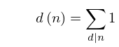
… ►It is the special case $k=2$ of the function $d_k\left(n\right)$ that counts the number of ways of expressing $n$ as the product of $k$ factors, with the order of factors taken into account. …Note that ${\sigma }_0\left(n\right)=d\left(n\right)$. … ►Table 27.2.2 tabulates the Euler totient function $\varphi \left(n\right)$, the divisor function $d\left(n\right)$ ($={\sigma }_0(n)$), and the sum of the divisors $\sigma (n)$ ($={\sigma }_1(n)$), for $n=1(1)52$. … ►

Table 27.2.2: Functions related to division.

► ►►►

$n$	$\varphi \left(n\right)$	$d\left(n\right)$	$\sigma \left(n\right)$	$n$	$\varphi \left(n\right)$	$d\left(n\right)$	$\sigma \left(n\right)$	$n$	$\varphi \left(n\right)$	$d\left(n\right)$	$\sigma \left(n\right)$	$n$	$\varphi \left(n\right)$	$d\left(n\right)$	$\sigma \left(n\right)$
…
10	4	4	18	23	22	2	24	36	12	9	91	49	42	3	57
…

►

25: 23.20 Mathematical Applications

… ►An algebraic curve that can be put either into the form … ►Given $P$, calculate $2P$, $4P$, $8P$ by doubling as above. …If any of $2P$, $4P$, $8P$ is not an integer, then the point has infinite order. Otherwise observe any equalities between $P$, $2P$, $4P$, $8P$, and their negatives. The order of a point (if finite and not already determined) can have only the values 3, 5, 6, 7, 9, 10, or 12, and so can be found from $2P=-P$, $4P=-P$, $4P=-2P$, $8P=P$, $8P=-P$, $8P=-2P$, or $8P=-4P$. …

26: 3.5 Quadrature

… ►If in addition $f$ is periodic, $f\in C^k(ℝ)$, and the integral is taken over a period, then … ►If $f\in C^{2m+2}[a,b]$, then the remainder $E_n(f)$ in (3.5.2) can be expanded in the form … ►About $2^9=512$ function evaluations are needed. … ►For further information, see Mason and Handscomb (2003, Chapter 8), Davis and Rabinowitz (1984, pp. 74–92), and Clenshaw and Curtis (1960). … ►For $C^{\mathrm{\infty }}$ functions Gauss quadrature can be very efficient. …

27: Software Index

… ► ►►►►►►►

	Open Source													With Book						Commercial
…
8 Incomplete Gamma and Related Functions
…
9 Airy and Related Functions
…
19.39(iii) $F(\varphi ,k)$, $E(\varphi ,k)$, $\varphi ,k\in ℝ$	✓		✓		✓	✓		✓	✓			✓	✓			✓					✓	✓	a	✓
19.39(iv) $R_C(x,y)$, $R_F(x,y,z)$, $R_D(x,y,z)$, $R_J(x,y,z,p)$	✓				✓				✓		✓	a	✓			✓				✓				✓	Derive
…
34 3j, 6j, 9j Symbols
…

…

28: 19.37 Tables

… ►Tabulated for $\varphi =0(5^{\circ }){90}^{\circ }$, $k^2=0(.01)1$ to 10D by Fettis and Caslin (1964). ►Tabulated for $\varphi =0(1^{\circ }){90}^{\circ }$, $k^2=0(.01)1$ to 7S by Beli͡akov et al. (1962). … ►Tabulated for $\varphi =0(5^{\circ }){90}^{\circ }$, $k=0(.01)1$ to 10D by Fettis and Caslin (1964). ►Tabulated for $\varphi =0(5^{\circ }){90}^{\circ }$, $\arcsin k=0(1^{\circ }){90}^{\circ }$ to 6D by Byrd and Friedman (1971), for $\varphi =0(5^{\circ }){90}^{\circ }$, $\arcsin k=0(2^{\circ }){90}^{\circ }$ and $5^{\circ }({10}^{\circ }){85}^{\circ }$ to 8D by Abramowitz and Stegun (1964, Chapter 17), and for $\varphi =0({10}^{\circ }){90}^{\circ }$, $\arcsin k=0(5^{\circ }){90}^{\circ }$ to 9D by Zhang and Jin (1996, pp. 674–675). … ►Tabulated for $\varphi =5^{\circ }(5^{\circ }){80}^{\circ }({2.5}^{\circ }){90}^{\circ }$, ${\alpha }^2=-1(.1)-0.1,0.1(.1)1$, $k^2=0(.05)0.9(.02)1$ to 10D by Fettis and Caslin (1964) (and warns of inaccuracies in Selfridge and Maxfield (1958) and Paxton and Rollin (1959)). …

29: 18.6 Symmetry, Special Values, and Limits to Monomials

… ►

Table 18.6.1: Classical OP’s: symmetry and special values.

► ►►►

$p_n(x)$	$p_n(-x)$	$p_n(1)$	$p_{2n}(0)$	$p_{2n+1}^{\prime }(0)$
…
$C_n^{(\lambda )}\left(x\right)$	${(-1)}^n{C}_n^{(\lambda )}\left(x\right)$	${\left(2\lambda \right)}_n/n!$	${(-1)}^n{\left(\lambda \right)}_n/n!$	$2{(-1)}^n{\left(\lambda \right)}_{n+1}/n!$
…

►

… ►

18.6.4 $$\underset{\lambda \to \mathrm{\infty }}{lim}\frac{C_n^{(\lambda )}\left(x\right)}{C_n^{(\lambda )}\left(1\right)}=x^n,$$

ⓘ

Symbols:

$C_n^{(\lambda )}\left(x\right)$: ultraspherical (or Gegenbauer) polynomial, $n$: nonnegative integer and $x$: real variable

Referenced by:

§18.18(iv), §18.6(ii)

Permalink:

http://dlmf.nist.gov/18.6.E4

Encodings:

pMML, png, TeX

See also:

Annotations for §18.6(ii), §18.6 and Ch.18

…

30: 26.3 Lattice Paths: Binomial Coefficients

… ►

Table 26.3.1: Binomial coefficients $\left(\genfrac{}{}{0.0pt}{}{m}{n}\right)$.

► ►►►►►

$m$	$n$
	0	1	2	3	4	5	6	7	8	9	10
…
8	1	8	28	56	70	56	28	8	1
9	1	9	36	84	126	126	84	36	9	1
…

►

►

Table 26.3.2: Binomial coefficients $\left(\genfrac{}{}{0.0pt}{}{m+n}{m}\right)$ for lattice paths.

► ►►►►

$m$	$n$
	…
1	1	2	3	4	5	6	7	8	9
…
8	1	9	45	165	495	1287	3003	6435	12870

►

…