values at q=0

SearchAdvancedHelp

(0.003 seconds)

11—20 of 58 matching pages

11: 2.4 Contour Integrals

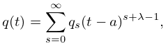
… ►Except that $\lambda$ is now permitted to be complex, with $\mathrm{\Re }\lambda >0$, we assume the same conditions on $q(t)$ and also that the Laplace transform in (2.3.8) converges for all sufficiently large values of $\mathrm{\Re }z$. … ►

In a neighborhood of $a$

2.4.11

$$p(t)=p(a)+\sum _{s=0}^{\mathrm{\infty }}{p}_s{(t-a)}^{s+\mu },$$

$$q(t)=\sum _{s=0}^{\mathrm{\infty }}{q}_s{(t-a)}^{s+\lambda -1},$$

ⓘ

Symbols:

$\lambda$: constant, $a$: left endpoint, $p(t)$: analytic function, $q(t)$: analytic function, $p_s$: coefficients, $q_s$: coefficients and $\mu$: positive constant

Referenced by:

§2.4(iv)

Permalink:

http://dlmf.nist.gov/2.4.E11

Encodings:

pMML, pMML, png, png, TeX, TeX

See also:

Annotations for §2.4(iii), §2.4 and Ch.2

with $\mathrm{\Re }\lambda >0$, $\mu >0$, $p_0\ne 0$, and the branches of ${(t-a)}^{\lambda }$ and ${(t-a)}^{\mu }$ continuous and constructed with $\mathrm{ph}\left(t-a\right)\to \omega$ as $t\to a$ along $𝒫$.

… ►and apply the result of §2.4(iii) to each integral on the right-hand side, the role of the series (2.4.11) being played by the Taylor series of $p(t)$ and $q(t)$ at $t=t_0$. … ►Cases in which $p^{\prime }(t_0)\ne 0$ are usually handled by deforming the integration path in such a way that the minimum of $\mathrm{\Re }\left(zp(t)\right)$ is attained at a saddle point or at an endpoint. … ►with $p,q$ and their derivatives evaluated at $t_0$. …

12: 28.13 Graphics

… ►

§28.13(i) Eigenvalues ${\lambda }_{\nu }\left(q\right)$ for General $\nu$

►

►►

Figure 28.13.1: ${\lambda }_{\nu }\left(q\right)$ as a function of $q$ for $\nu =0.5(1)3.5$ and $a_n\left(q\right),b_n\left(q\right)$ for $n=0,1,2,3,4$ ($a$’s), $n=1,2,3,4$ ($b$’s). … Magnify

►

►

►

Figure 28.13.2: ${\lambda }_{\nu }\left(q\right)$ for , $0\le q\le 10$. Magnify 3D Help

►

§28.13(ii) Solutions ${\mathrm{ce}}_{\nu }(x,q)$, ${\mathrm{se}}_{\nu }(x,q)$, and ${\mathrm{me}}_{\nu }(x,q)$ for General $\nu$

… ►

►

►

Figure 28.13.4: ${\mathrm{se}}_{\nu }(x,1)$ for , $0\le x\le 2\pi$. Magnify 3D Help

…

13: 2.3 Integrals of a Real Variable

… ►Assume that $q(t)$ again has the expansion (2.3.7) and this expansion is infinitely differentiable, $q(t)$ is infinitely differentiable on $(0,\mathrm{\infty })$, and each of the integrals $\int {\mathrm{e}}^{\mathrm{i}xt}{q}^{(s)}(t)dt$, $s=0,1,2,\mathrm{\dots }$, converges at $t=\mathrm{\infty }$, uniformly for all sufficiently large $x$. … ►Assume also that ${\partial }^{2}p(\alpha ,t)/{\partial t}^2$ and $q(\alpha ,t)$ are continuous in $\alpha$ and $t$, and for each $\alpha$ the minimum value of $p(\alpha ,t)$ in $[0,k)$ is at $t=\alpha$, at which point $\partial p(\alpha ,t)/\partial t$ vanishes, but both ${\partial }^{2}p(\alpha ,t)/{\partial t}^2$ and $q(\alpha ,t)$ are nonzero. … ► $\kappa =\kappa (\alpha )$ being the value of $w$ at $t=k$. We now expand $f(\alpha ,w)$ in a Taylor series centered at the peak value $w=a$ of the exponential factor in the integrand: …with the coefficients ${\varphi }_s(\alpha )$ continuous at $\alpha =0$. …

14: 28.12 Definitions and Basic Properties

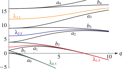
… ►For given $\nu$ (or $\cos \left(\nu \pi \right)$) and $q$, equation (28.2.16) determines an infinite discrete set of values of $a$, denoted by ${\lambda }_{\nu +2n}\left(q\right)$, $n=0,\pm 1,\pm 2,\mathrm{\dots }$. … ►As a function of $\nu$ with fixed $q$ ($\ne 0$), ${\lambda }_{\nu }\left(q\right)$ is discontinuous at $\nu =\pm 1,\pm 2,\mathrm{\dots }$. … ►However, these functions are not the limiting values of ${\mathrm{me}}_{\pm \nu }(z,q)$ as $\nu \to n$ $(\ne 0)$. … ►These functions are real-valued for real $\nu$, real $q$, and $z=x$, whereas ${\mathrm{me}}_{\nu }(x,q)$ is complex. … ►Again, the limiting values of ${\mathrm{ce}}_{\nu }(z,q)$ and ${\mathrm{se}}_{\nu }(z,q)$ as $\nu \to n$ $(\ne 0)$ are not the functions ${\mathrm{ce}}_n(z,q)$ and ${\mathrm{se}}_n(z,q)$ defined in §28.2(vi). …

15: 28.33 Physical Applications

… ►where $q=\frac{1}{4}{c}^2{k}^2$ and $a_n(q)$ or $b_n(q)$ is the separation constant; compare (28.12.11), (28.20.11), and (28.20.12). …The boundary conditions for $\xi ={\xi }_0$ (outer clamp) and $\xi ={\xi }_1$ (inner clamp) yield the following equation for $q$: … ►As $\omega$ runs from $0$ to $+\mathrm{\infty }$, with $b$ and $f$ fixed, the point $(q,a)$ moves from $\mathrm{\infty }$ to $0$ along the ray $ℒ$ given by the part of the line $a=(2b/f)q$ that lies in the first quadrant of the $(q,a)$-plane. … ►For points $(q,a)$ that are at intersections of $ℒ$ with the characteristic curves $a=a_n\left(q\right)$ or $a=b_n\left(q\right)$, a periodic solution is possible. … ►References for other initial-value problems include: …

16: 8.3 Graphics

… ►In the graphics shown in this subsection, height corresponds to the absolute value of the function and color to the phase. … ►

►

►

Figure 8.3.8: $\mathrm{\Gamma }(0.25,x+\mathrm{i}y)$, $-3\le x\le 3$, $-3\le y\le 3$. Principal value. … Magnify 3D Help

►

►

►

Figure 8.3.9: $\gamma (0.25,x+\mathrm{i}y)$, $-3\le x\le 3$, $-3\le y\le 3$. Principal value. … Magnify 3D Help

… ►

►

►

Figure 8.3.14: $\mathrm{\Gamma }(2.5,x+\mathrm{i}y)$, $-2.2\le x\le 3$, $-3\le y\le 3$. Principal value. … Magnify 3D Help

►

►

►

Figure 8.3.15: $\gamma (2.5,x+\mathrm{i}y)$, $-2.2\le x\le 3$, $-3\le y\le 3$. Principal value. … Magnify 3D Help

…

17: About Color Map

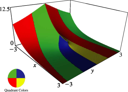
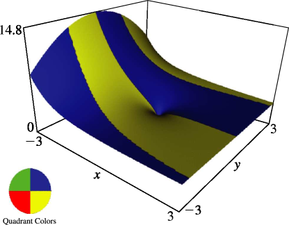
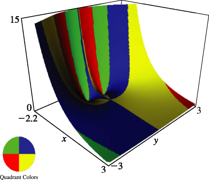
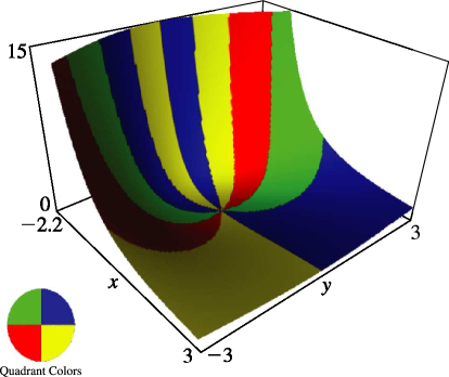
… ►By painting the surfaces with a color that encodes the phase, $\mathrm{ph}f$, both the magnitude and phase of complex valued functions can be displayed. … ►In doing this, however, we would like to place the mathematically significant phase values, specifically the multiples of $\pi /2$ correponding to the real and imaginary axes, at more immediately recognizable colors. … ►The conventional CMYK color wheel (not to be confused with the traditional Artist’s color wheel) places the additive colors (red, green, blue) and the subtractive colors (yellow, cyan, magenta) at multiples of 60 degrees. In particular, the colors at 90 and 180 degrees are some vague greenish and purplish hues. … ►Specifically, by scaling the phase angle in $[0,2\pi )$ to $q$ in the interval $[0,4)$, the hue (in degrees) is computed as …

18: 14.21 Definitions and Basic Properties

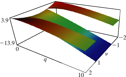
… ► $P_{\nu }^{\pm \mu }\left(z\right)$ and ${𝑸}_{\nu }^{\mu }\left(z\right)$ exist for all values of $\nu$, $\mu$, and $z$, except possibly $z=\pm 1$ and $\mathrm{\infty }$, which are branch points (or poles) of the functions, in general. When $z$ is complex $P_{\nu }^{\pm \mu }\left(z\right)$, $Q_{\nu }^{\mu }\left(z\right)$, and ${𝑸}_{\nu }^{\mu }\left(z\right)$ are defined by (14.3.6)–(14.3.10) with $x$ replaced by $z$: the principal branches are obtained by taking the principal values of all the multivalued functions appearing in these representations when $z\in (1,\mathrm{\infty })$, and by continuity elsewhere in the $z$-plane with a cut along the interval $(-\mathrm{\infty },1]$; compare §4.2(i). 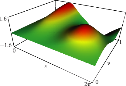… … ►When $\mathrm{\Re }\nu \ge -\frac{1}{2}$ and $\mathrm{\Re }\mu \ge 0$, a numerically satisfactory pair of solutions of (14.21.1) in the half-plane $|\mathrm{ph}z|\le \frac{1}{2}\pi$ is given by $P_{\nu }^{-\mu }\left(z\right)$ and ${𝑸}_{\nu }^{\mu }\left(z\right)$. ►

§14.21(iii) Properties

…

19: 14.28 Sums

… ►When $\mathrm{\Re }{z}_1>0$, $\mathrm{\Re }{z}_2>0$, , and , ►

14.28.1 $$P_{\nu }\left(z_1{z}_2-{\left(z_1^2-1\right)}^{1/2}{\left(z_2^2-1\right)}^{1/2}\cos \varphi \right)=P_{\nu }\left(z_1\right)P_{\nu }\left(z_2\right)+2\sum _{m=1}^{\mathrm{\infty }}{(-1)}^m\frac{\mathrm{\Gamma }\left(\nu -m+1\right)}{\mathrm{\Gamma }\left(\nu +m+1\right)}{P}_{\nu }^m\left(z_1\right)P_{\nu }^m(z_2)\cos \left(m\varphi \right),$$

ⓘ

Symbols:

$\mathrm{\Gamma }\left(z\right)$: gamma function, $P_{\nu }^{\mu }\left(z\right)$: associated Legendre function of the first kind, $\cos z$: cosine function, $P_{\nu }\left(z\right)=P_{\nu }^0\left(z\right)$: Legendre function of the first kind, $z$: complex variable, $m$: nonnegative integer and $\nu$: general degree

Permalink:

http://dlmf.nist.gov/14.28.E1

Encodings:

pMML, png, TeX

See also:

Annotations for §14.28(i), §14.28 and Ch.14

►where the branches of the square roots have their principal values when $z_1,z_2\in (1,\mathrm{\infty })$ and are continuous when $z_1,z_2\in ℂ\setminus (0,1]$. … ►

14.28.2 $$\sum _{n=0}^{\mathrm{\infty }}(2n+1)Q_n\left(z_1\right)P_n\left(z_2\right)=\frac{1}{z_1-z_2},$$ $z_1\in {ℰ}_1$, $z_2\in {ℰ}_2$,

ⓘ

Symbols:

$\in$: element of, $P_{\nu }\left(z\right)=P_{\nu }^0\left(z\right)$: Legendre function of the first kind, $Q_{\nu }\left(z\right)=Q_{\nu }^0\left(z\right)$: Legendre function of the second kind, $z$: complex variable, $n$: nonnegative integer and ${ℰ}_1$, ${ℰ}_2$: ellipses

Permalink:

http://dlmf.nist.gov/14.28.E2

Encodings:

pMML, png, TeX

See also:

Annotations for §14.28(ii), §14.28 and Ch.14

►where ${ℰ}_1$ and ${ℰ}_2$ are ellipses with foci at $\pm 1$, ${ℰ}_2$ being properly interior to ${ℰ}_1$. …

20: 13.4 Integral Representations

… ►The contour of integration starts and terminates at a point $\alpha$ on the real axis between $0$ and $1$. …The fractional powers are continuous and assume their principal values at $t=\alpha$. …At the point where the contour crosses the interval $(1,\mathrm{\infty })$, $t^{-b}$ and the ${}_2{}^{}𝐅_1^{}$ function assume their principal values; compare §§15.1 and 15.2(i). …At this point the fractional powers are determined by $\mathrm{ph}t=\pi$ and $\mathrm{ph}\left(1+t\right)=0$. 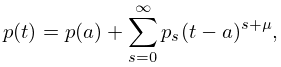… ►If $a\ne 0,-1,-2,\mathrm{\dots }$, then …