graphical interpretation via Glaisher notation

SearchAdvancedHelp

(0.002 seconds)

11—20 of 405 matching pages

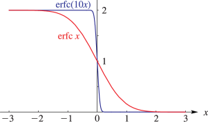
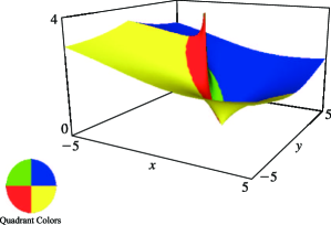
11: 7.3 Graphics

§7.3 Graphics

… ►

►►

Figure 7.3.1: Complementary error functions $\mathrm{erfc}x$ and $\mathrm{erfc}\left(10x\right)$, $-3\le x\le 3$. Magnify

►

►►

Figure 7.3.2: Dawson’s integral $F\left(x\right)$, $-3.5\le x\le 3.5$. Magnify

… ►

►

►

Figure 7.3.5: $|\mathrm{erf}\left(x+\mathrm{i}y\right)|$, $-3\le x\le 3$, $-3\le y\le 3$. … Magnify 3D Help

►

►

►

Figure 7.3.6: $|\mathrm{erfc}\left(x+\mathrm{i}y\right)|$, $-3\le x\le 3$, $-3\le y\le 3$. … Magnify 3D Help

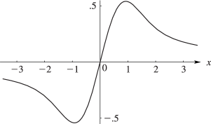
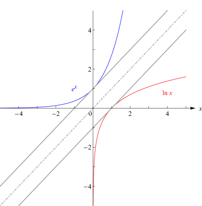
12: 4.3 Graphics

§4.3 Graphics

… ►

►►

Figure 4.3.1: $\ln x$ and ${\mathrm{e}}^x$. … Magnify

… ►In the graphics shown in this subsection height corresponds to the absolute value of the function and color to the phase. … ►

►

►

Figure 4.3.3: $\ln \left(x+\mathrm{i}y\right)$ (principal value). … Magnify 3D Help

►

►

►

Figure 4.3.4: ${\mathrm{e}}^{x+\mathrm{i}y}$. Magnify 3D Help

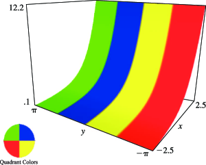
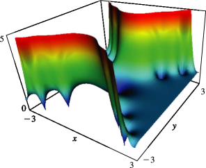
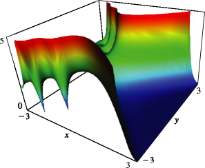
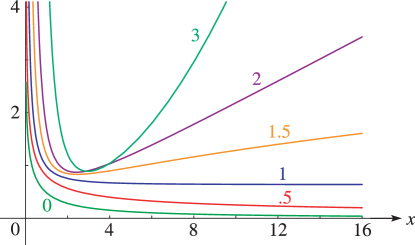
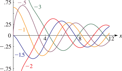
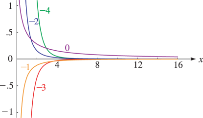
13: 11.3 Graphics

§11.3 Graphics

… ►

►►

Figure 11.3.1: ${𝐇}_{\nu }\left(x\right)$ for $0\le x\le 12$ and $\nu =0,\frac{1}{2},1,\frac{3}{2},2,3$. Magnify

►

►►

Figure 11.3.2: ${𝐊}_{\nu }\left(x\right)$ for and $\nu =0,\frac{1}{2},1,\frac{3}{2},2,3$. Magnify

►

►►

Figure 11.3.3: ${𝐇}_{\nu }\left(x\right)$ for $0\le x\le 12$ and $\nu =-3,-2,-\frac{3}{2},-1,-\frac{1}{2}$. Magnify

►

►►

Figure 11.3.4: ${𝐊}_{\nu }\left(x\right)$ for and $\nu =-4,-3,-2,-1,0$. … Magnify

…

14: DLMF Project News

error generating summary

15: Viewing DLMF Interactive 3D Graphics

Viewing DLMF Interactive 3D Graphics

… ►WebGL is a JavaScript API (application programming interface) for rendering 3D graphics in a web browser without the use of a plugin. Our WebGL code is based on the X3DOM framework which allows the building of the WebGL application around X3D, an XML based graphics code. … ►” VRML (Virtual Reality Modeling Language) is a standard file format for viewing 3D graphics on the web and X3D is its successor. …

16: 10.26 Graphics

§10.26 Graphics

►

§10.26(i) Real Order and Variable

… ►For the notation, see §10.45. …

17: 23.16 Graphics

§23.16 Graphics

…

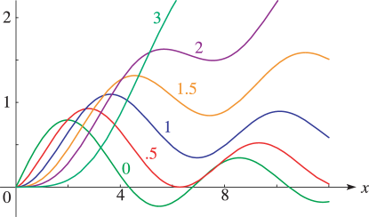
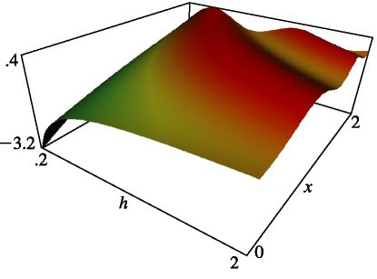
18: 28.21 Graphics

§28.21 Graphics

►

Radial Mathieu Functions: Surfaces

… ►

►

►

Figure 28.21.6: ${\mathrm{Ms}}_1^{(2)}(x,h)$ for $0.2\le h\le 2$, $0\le x\le 2$. Magnify 3D Help

19: 18.40 Methods of Computation

… ►

Stieltjes Inversion via (approximate) Analytic Continuation

… ►Gautschi (2004, p. 119–120) has explored the $\epsilon \to 0^{+}$ limit via the Wynn $\epsilon$-algorithm, (3.9.11) to accelerate convergence, finding four to eight digits of precision in $w(x)$, depending smoothly on $x^{\prime }$, for $N\approx 4000$, for an example involving first numerator Legendre OP’s. … ►The bottom and top of the steps at the $x_i$ are lower and upper bounds to ${\int }_a^{x_i}d\mu (x)$ as made explicit via the Chebyshev inequalities discussed by Shohat and Tamarkin (1970, pp. 42–43). … ►In what follows this is accomplished in two ways: i) via the Lagrange interpolation of §3.3(i) ; and ii) by constructing a pointwise continued fraction, or PWCF, as follows: …where the coefficients are defined recursively via $a_1=\frac{x_{1,N}}{x_{2,N}}-1$, and …

20: 28.12 Definitions and Basic Properties

… ►

§28.12(i) Eigenvalues ${\lambda }_{\nu +2n}\left(q\right)$

… ►For graphical interpretation see Figure 28.13.1. …