.足球世界杯开球_『wn4.com_』世界杯输了要赔钱吗_w6n2c9o_2022年11月29日2时54分22秒_ic6k0s0ic
(0.004 seconds)
11—20 of 789 matching pages
11: 24.2 Definitions and Generating Functions
12: 3.7 Ordinary Differential Equations
…
►The path is partitioned at points labeled successively , with , .
…
►Write , , expand and in Taylor series (§1.10(i)) centered at , and apply (3.7.2).
…
►If, for example, , then on moving the contributions of and to the right-hand side of (3.7.13) the resulting system of equations is not tridiagonal, but can readily be made tridiagonal by annihilating the elements of that lie below the main diagonal and its two adjacent diagonals.
…
►The values are the eigenvalues and the corresponding solutions of the differential equation are the eigenfunctions.
…
►where and
…
13: 3.2 Linear Algebra
…
►where , , , and
…Forward elimination for solving then becomes ,
…and back substitution is , followed by
…
►Define the Lanczos vectors
and coefficients and by , a normalized vector (perhaps chosen randomly), , , and for by the recursive scheme
…
►Start with , vector such that , , .
…
14: 28.6 Expansions for Small
…
►Leading terms of the power series for and for are:
…
►The coefficients of the power series of , and also , are the same until the terms in and , respectively.
…
►Numerical values of the radii of convergence of the power series (28.6.1)–(28.6.14) for are given in Table 28.6.1.
Here for , for , and for and .
…
►
§28.6(ii) Functions and
…15: 26.12 Plane Partitions
…
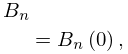
►
26.12.9
…
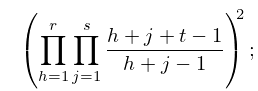
►
26.12.10
…
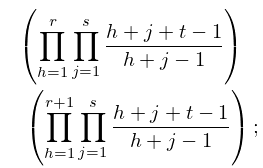
►
26.12.11
…
►The notation denotes the sum over all plane partitions contained in , and denotes the number of elements in .
…
►where is the sum of the squares of the divisors of .
…
16: 10.75 Tables
…
►
•
…
►
•
…
►
•
…
►
•
…
►
•
…
Achenbach (1986) tabulates , , , , , 20D or 18–20S.
Makinouchi (1966) tabulates all values of and in the interval , with at least 29S. These are for , 10, 20; , ; with and , except for .
Abramowitz and Stegun (1964, Chapter 11) tabulates , , , 10D; , , , 8D.
Leung and Ghaderpanah (1979), tabulates all zeros of the principal value of , for , 29S.
Abramowitz and Stegun (1964, Chapter 11) tabulates , , , 7D; , , , 6D.
17: 19.29 Reduction of General Elliptic Integrals
…
►Let
…where
…
►Next, for , define , and assume both ’s are positive for .
…where
…If , where both linear factors are positive for , and , then (19.29.25) is modified so that
…
18: 3.6 Linear Difference Equations
…
►Given numerical values of and , the solution of the equation
…These errors have the effect of perturbing the solution by unwanted small multiples of and of an independent solution , say.
…
►The unwanted multiples of now decay in comparison with , hence are of little consequence.
…
►The latter method is usually superior when the true value of is zero or pathologically small.
…
►beginning with .
…
19: 5.10 Continued Fractions
20: 3.9 Acceleration of Convergence
…
►A transformation of a convergent sequence with limit into a sequence is called limit-preserving if converges to the same limit .
…
►This transformation is accelerating if is a linearly convergent
sequence, i.
…
►Then the transformation of the sequence into a sequence is given by
…
►Then .
…
►We give a special form of Levin’s transformation in which the sequence of partial sums is transformed into:
…
