.世界杯赌挣钱吗盘_『wn4.com_』澳门赛的抽签出来了吗_w2n3c1o_2022年12月10日16时43分54秒_eeyyrupg4_gov_hk

SearchAdvancedHelp

(0.006 seconds)

11—20 of 805 matching pages

11: 23.9 Laurent and Other Power Series

… ►Let $z_0(\ne 0)$ be the nearest lattice point to the origin, and define …Explicit coefficients $c_n$ in terms of $c_2$ and $c_3$ are given up to $c_{19}$ in Abramowitz and Stegun (1964, p. 636). ►For $j=1,2,3$, and with $e_j$ as in §23.3(i), … ►where $a_{0,0}=1$, $a_{m,n}=0$ if either $m$ or , and …For $a_{m,n}$ with $m=0,1,\mathrm{\dots },12$ and $n=0,1,\mathrm{\dots },8$, see Abramowitz and Stegun (1964, p. 637).

12: 32.3 Graphics

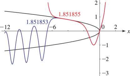
… ►Plots of solutions $w_k(x)$ of ${\text{P}}_{\text{I}}$ with $w_k(0)=0$ and $w_k^{\prime }(0)=k$ for various values of $k$, and the parabola $6w^2+x=0$. … ►

►►

Figure 32.3.3: $w_k(x)$ for $-12\le x\le 0.73$ and $k=\mathrm{1.85185\hspace{0.33em}3}$, $\mathrm{1.85185\hspace{0.33em}5}$. … Magnify

… ►Here $w_k(x)$ is the solution of ${\text{P}}_{\text{II}}$ with $\alpha =0$ and such that … ►Here $u=u_k(x;\nu )$ is the solution of …The corresponding solution of ${\text{P}}_{\text{IV}}$ is given by …

13: 3.9 Acceleration of Convergence

… ►A transformation of a convergent sequence $\{s_n\}$ with limit $\sigma$ into a sequence $\{t_n\}$ is called limit-preserving if $\{t_n\}$ converges to the same limit $\sigma$. … ►Then the transformation of the sequence $\{s_n\}$ into a sequence $\{t_{n,2k}\}$ is given by … ►Then $t_{n,2k}={\epsilon }_{2k}^{(n)}$. … ►with $s_{\mathrm{\infty }}=\frac{1}{12}{\pi }^2=\mathrm{0.82246\hspace{0.33em}70334\hspace{0.33em}24}\mathrm{\dots }$. … ►We give a special form of Levin’s transformation in which the sequence $s=\{s_n\}$ of partial sums $s_n={\sum }_{j=0}^n{a}_j$ is transformed into: …

14: 11.14 Tables

… ►

Abramowitz and Stegun (1964, Chapter 12) tabulates ${𝐇}_n\left(x\right)$, ${𝐇}_n\left(x\right)-Y_n\left(x\right)$, and $I_n\left(x\right)-{𝐋}_n\left(x\right)$ for $n=0,1$ and $x=0(.1)5$, $x^{-1}=0(.01)0.2$ to 6D or 7D.

… ►

Barrett (1964) tabulates ${𝐋}_n\left(x\right)$ for $n=0,1$ and $x=0.2(.005)4(.05)10(.1)19.2$ to 5 or 6S, $x=6(.25)59.5(.5)100$ to 2S.

… ►

Abramowitz and Stegun (1964, Chapter 12) tabulates ${\int }_0^x(I_0\left(t\right)-{𝐋}_0\left(t\right))dt$ and $(2/\pi ){\int }_x^{\mathrm{\infty }}{t}^{-1}{𝐇}_0\left(t\right)dt$ for $x=0(.1)5$ to 5D or 7D; ${\int }_0^x({𝐇}_0\left(t\right)-Y_0\left(t\right))dt-(2/\pi )\ln x$, ${\int }_0^x(I_0\left(t\right)-{𝐋}_0\left(t\right))dt-(2/\pi )\ln x$, and ${\int }_x^{\mathrm{\infty }}{t}^{-1}({𝐇}_0\left(t\right)-Y_0\left(t\right))dt$ for $x^{-1}=0(.01)0.2$ to 6D.

… ►

Bernard and Ishimaru (1962) tabulates ${𝐉}_{\nu }\left(x\right)$ and ${𝐄}_{\nu }\left(x\right)$ for $\nu =-10(.1)10$ and $x=0(.1)10$ to 5D.

… ►

Agrest and Maksimov (1971, Chapter 11) defines incomplete Struve, Anger, and Weber functions and includes tables of an incomplete Struve function ${𝐇}_n\left(x,\alpha \right)$ for $n=0,1$, $x=0(.2)10$, and $\alpha =0(.2)1.4,\frac{1}{2}\pi$, together with surface plots.

15: 24.2 Definitions and Generating Functions

… ►

$B_{2n+1}=0$ ,

… ►

24.2.4 $$B_n=B_n\left(0\right),$$

ⓘ

Symbols:

$B_n$: Bernoulli numbers, $B_n\left(x\right)$: Bernoulli polynomials and $n$: integer

A&S Ref:

23.1.2

Referenced by:

(25.11.7)

Permalink:

http://dlmf.nist.gov/24.2.E4

Encodings:

pMML, png, TeX

See also:

Annotations for §24.2(i), §24.2 and Ch.24

… ►

Table 24.2.4: Euler numbers $E_n$.

► ►►

$n$	$E_n$
…

►

►

Table 24.2.5: Coefficients $b_{n,k}$ of the Bernoulli polynomials $B_n\left(x\right)={\sum }_{k=0}^n{b}_{n,k}{x}^k$.

► ►►

	$k$
…

►

►

Table 24.2.6: Coefficients $e_{n,k}$ of the Euler polynomials $E_n\left(x\right)={\sum }_{k=0}^n{e}_{n,k}{x}^k$.

► ►►

	$k$
…

►

16: 27.2 Functions

… ►where $p_1,p_2,\mathrm{\dots },p_{\nu \left(n\right)}$ are the distinct prime factors of $n$, each exponent $a_r$ is positive, and $\nu \left(n\right)$ is the number of distinct primes dividing $n$. … ►Note that ${\sigma }_0\left(n\right)=d\left(n\right)$. …Note that $J_1\left(n\right)=\varphi \left(n\right)$. ►In the following examples, $a_1,\mathrm{\dots },a_{\nu \left(n\right)}$ are the exponents in the factorization of $n$ in (27.2.1). … ►Table 27.2.1 lists the first 100 prime numbers $p_n$. …

17: 1.3 Determinants, Linear Operators, and Spectral Expansions

… ►The cofactor $A_{jk}$ of $a_{jk}$ is … ►For real-valued $a_{jk}$, … ►where ${\omega }_1,{\omega }_2,\mathrm{\dots },{\omega }_n$ are the $n$th roots of unity (1.11.21). … ►If ${𝐷}_n[a_{j,k}]$ tends to a limit $L$ as $n\to \mathrm{\infty }$, then we say that the infinite determinant ${𝐷}_{\mathrm{\infty }}[a_{j,k}]$ converges and ${𝐷}_{\mathrm{\infty }}[a_{j,k}]=L$. … ►The corresponding eigenvectors ${𝐚}_1,\mathrm{\dots },{𝐚}_n$ can be chosen such that they form a complete orthonormal basis in ${𝐄}_n$. …

18: 3.2 Linear Algebra

… ►where $u_j=c_j$, $j=1,2,\mathrm{\dots },n-1$, $d_1=b_1$, and …Forward elimination for solving $𝐀𝐱=𝐟$ then becomes $y_1=f_1$, …and back substitution is $x_n=y_n/d_n$, followed by … ►Define the Lanczos vectors ${𝐯}_j$ and coefficients ${\alpha }_j$ and ${\beta }_j$ by ${𝐯}_0=\mathrm{𝟎}$, a normalized vector ${𝐯}_1$ (perhaps chosen randomly), ${\alpha }_1={𝐯}_1^{\mathrm{T}}𝐀{𝐯}_1$, ${\beta }_1=0$, and for $j=1,2,\mathrm{\dots },n-1$ by the recursive scheme … ►Start with ${𝐯}_0=\mathrm{𝟎}$, vector ${𝐯}_1$ such that ${𝐯}_1^{\mathrm{T}}𝐒{𝐯}_1=1$, ${\alpha }_1={𝐯}_1^{\mathrm{T}}𝐀{𝐯}_1$, ${\beta }_1=0$. …

19: 3.10 Continued Fractions

… ►For instance, if none of the $u_n$ vanish, then we can define … ►The first two columns in this table are defined by …where the $c_n$ ($\ne 0$) appear in (3.10.7). … ►The $A_n$ and $B_n$ of (3.10.2) can be computed by means of three-term recurrence relations (1.12.5). … ►Then $u_0=C_n$. …

20: 10.48 Graphs

… ►

►►

Figure 10.48.1: ${𝗃}_n\left(x\right)$, $n=0(1)4$, $0\le x\le 12$. Magnify

►

►►

Figure 10.48.2: ${𝗒}_n\left(x\right)$, $n=0(1)4$, . Magnify

►

►►

Figure 10.48.3: ${𝗃}_5\left(x\right)$, ${𝗒}_5\left(x\right)$, $\sqrt{{𝗃}_5^2\left(x\right)+{𝗒}_5^2\left(x\right)}$, $0\le x\le 12$. Magnify

►

►►

Figure 10.48.4: ${𝗃}_5^{\prime }\left(x\right)$, ${𝗒}_5^{\prime }\left(x\right)$, $\sqrt{𝗃_5^{\prime }{}_{}{}^2\left(x\right)+𝗒_5^{\prime }{}_{}{}^2\left(x\right)}$, $0\le x\le 12$. Magnify

►

►►

Figure 10.48.5: ${𝗂}_0^{(1)}\left(x\right)$, ${𝗂}_0^{(2)}\left(x\right)$, ${𝗄}_0\left(x\right)$, $0\le x\le 4$. Magnify

…