§28.31 Equations of Whittaker–Hill and Ince
Contents
- §28.31(i) Whittaker–Hill Equation
- §28.31(ii) Equation of Ince; Ince Polynomials
- §28.31(iii) Paraboloidal Wave Functions
§28.31(i) Whittaker–Hill Equation
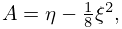
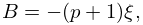
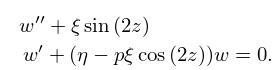
§28.31(ii) Equation of Ince; Ince Polynomials
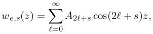
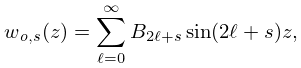
Formal -periodic solutions can be constructed as Fourier series; compare §28.4:
| 28.31.4 | ||||
| , | ||||
| 28.31.5 | ||||
| , | ||||
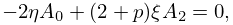
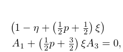
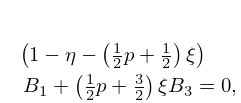
where the coefficients satisfy
| 28.31.6 | ||||
| , | ||||
| 28.31.7 | ||||
| , | ||||
| 28.31.8 | ||||
| , | ||||
| 28.31.9 | ||||
| . | ||||
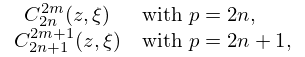
When is a nonnegative integer, the parameter can be chosen so that solutions of (28.31.3) are trigonometric polynomials, called Ince polynomials. They are denoted by
| 28.31.10 | |||
| 28.31.11 | |||
and in all cases.
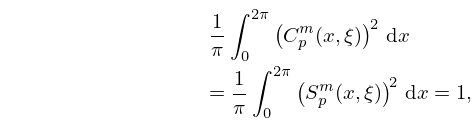
The values of corresponding to , are denoted by , , respectively. They are real and distinct, and can be ordered so that and have precisely zeros, all simple, in . The normalization is given by
| 28.31.12 | |||
ambiguities in sign being resolved by requiring and to be continuous functions of and positive when .
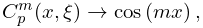
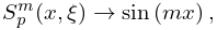
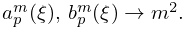
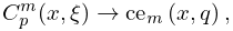
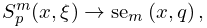
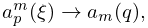
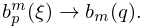
For , with fixed,
| 28.31.13 | ||||
| ; | ||||
§28.31(iii) Paraboloidal Wave Functions
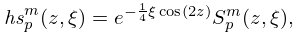
With (28.31.10) and (28.31.11),
| 28.31.16 | |||
| 28.31.17 | |||
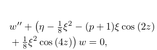
are called paraboloidal wave functions. They satisfy the differential equation
| 28.31.18 | |||
with , , respectively.
For change of sign of ,
| 28.31.19 | ||||
and
| 28.31.20 | ||||
For ,
| 28.31.21 | |||
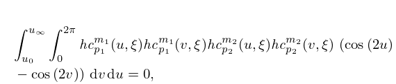
More important are the double orthogonality relations for or or both, given by
| 28.31.22 | |||
and
| 28.31.23 | |||
and also for all , given by
| 28.31.24 | |||
where when , and when .
Asymptotic Behavior
For , the functions , behave asymptotically as multiples of as . All other periodic solutions behave as multiples of .
For , the functions , behave asymptotically as multiples of as . All other periodic solutions behave as multiples of .
