two or more variables

SearchAdvancedHelp

(0.003 seconds)

21—30 of 286 matching pages

21: 4.24 Inverse Trigonometric Functions: Further Properties

… ►

4.24.2 $$\arccos z={(2(1-z))}^{1/2}\left(1+\sum _{n=1}^{\mathrm{\infty }}\frac{1\cdot 3\cdot 5\mathrm{\cdots }(2n-1)}{2^{2n}(2n+1)n!}{(1-z)}^n\right),$$ $|1-z|\le 2$.

ⓘ

Symbols:

$!$: factorial (as in $n!$), $\arccos z$: arccosine function, $n$: integer and $z$: complex variable

A&S Ref:

4.4.41 (which is stated differently and the constraint on $z$ is more restrictive.)

Permalink:

http://dlmf.nist.gov/4.24.E2

Encodings:

pMML, png, TeX

See also:

Annotations for §4.24(i), §4.24 and Ch.4

… ►which requires $z$ $(=x+\mathrm{i}y)$ to lie between the two rectangular hyperbolas given by …

22: 1.4 Calculus of One Variable

… ►For the functions discussed in the following DLMF chapters these two integration measures are adequate, as these special functions are analytic functions of their variables, and thus $C^{\mathrm{\infty }}$, and well defined for all values of these variables; possible exceptions being at boundary points. … ►Definite integrals over the Stieltjes measure $d\alpha (x)$ could represent a sum, an integral, or a combination of the two. …

23: 21.9 Integrable Equations

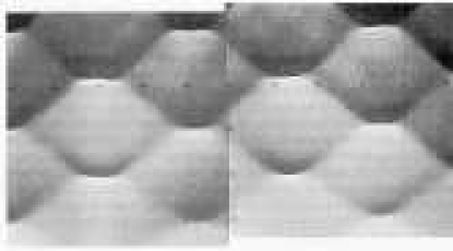
… ►Particularly important for the use of Riemann theta functions is the Kadomtsev–Petviashvili (KP) equation, which describes the propagation of two-dimensional, long-wave length surface waves in shallow water (Ablowitz and Segur (1981, Chapter 4)): … ►

►►

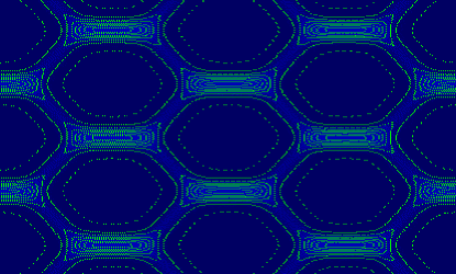
Figure 21.9.1: Two-dimensional periodic waves in a shallow water wave tank, taken from Hammack et al. (1995, p. 97) by permission of Cambridge University Press. The original caption reads “Mosaic of two overhead photographs, showing surface patterns of waves in shallow water. … Magnify

►

►►

Figure 21.9.2: Contour plot of a two-phase solution of Equation (21.9.3). Such a solution is given in terms of a Riemann theta function with two phases; see Krichever (1976), Dubrovin (1981), and Hammack et al. (1995). Magnify

…

24: 1.11 Zeros of Polynomials

… ►A monic polynomial of even degree with real coefficients has at least two zeros of opposite signs when the constant term is negative. … ►The number of positive zeros of a polynomial with real coefficients cannot exceed the number of times the coefficients change sign, and the two numbers have same parity. … ►

§1.11(iii) Polynomials of Degrees Two, Three, and Four

…

25: 18.32 OP’s with Respect to Freud Weights

… ►

18.32.1 $$w(x)=\exp \left(-Q(x)\right),$$ ,

ⓘ

Symbols:

$\exp z$: exponential function, $w(x)$: weight function and $x$: real variable

Referenced by:

§18.32

Permalink:

http://dlmf.nist.gov/18.32.E1

Encodings:

pMML, png, TeX

See also:

Annotations for §18.32 and Ch.18

… ►For asymptotic approximations to OP’s that correspond to Freud weights with more general functions $Q(x)$ see Deift et al. (1999a, b), Bleher and Its (1999), and Kriecherbauer and McLaughlin (1999). … ►

18.32.2 $$w(x)={\left|x\right|}^{\alpha }\exp \left(-Q(x)\right),$$ $x\in ℝ$, $\alpha >-1$,

ⓘ

Symbols:

$\in$: element of, $\exp z$: exponential function, $ℝ$: real line, $w(x)$: weight function and $x$: real variable

Referenced by:

§18.32, Erratum (V1.2.0) Section 18.32

Permalink:

http://dlmf.nist.gov/18.32.E2

Encodings:

pMML, png, TeX

Addition (effective with 1.2.0):

This equation was added.

See also:

Annotations for §18.32 and Ch.18

…

26: 13.5 Continued Fractions

… ►

13.5.1 $$\frac{M(a,b,z)}{M(a+1,b+1,z)}=1+\frac{u_{1}z}{1+}\frac{u_{2}z}{1+}\mathrm{\cdots },$$

ⓘ

Symbols:

$M(a,b,z)$: $={}_1{}^{}F_1^{}(a;b;z)$ Kummer confluent hypergeometric function, $z$: complex variable and $u_n$: continued fraction coefficients

Referenced by:

§13.31(ii)

Permalink:

http://dlmf.nist.gov/13.5.E1

Encodings:

pMML, png, TeX

See also:

Annotations for §13.5 and Ch.13

… ►For more details on how a continued fraction converges to a meromorphic function see Jones and Thron (1980). … ►

13.5.3 $$\frac{U(a,b,z)}{U(a,b-1,z)}=1+\frac{v_1/z}{1+}\frac{v_2/z}{1+}\mathrm{\cdots },$$

ⓘ

Symbols:

$U(a,b,z)$: Kummer confluent hypergeometric function, $z$: complex variable and $v_n$: continued fraction coefficients

Permalink:

http://dlmf.nist.gov/13.5.E3

Encodings:

pMML, png, TeX

See also:

Annotations for §13.5 and Ch.13

…

27: 19.20 Special Cases

… ►

19.20.19 $$R_D(x,y,z)\sim 3x^{-1/2}{y}^{-1/2}{z}^{-1/2},$$ $z/\sqrt{xy}\to 0$.

ⓘ

Symbols:

$R_D(x,y,z)$: elliptic integral symmetric in only two variables and $\sim$: asymptotic equality

Referenced by:

§19.20(iv), Erratum (V1.1.3) for Chapter 19

Permalink:

http://dlmf.nist.gov/19.20.E19

Encodings:

pMML, png, TeX

Correction (effective with 1.1.3):

The factors inside the square root on the right-hand side were written as products to ensure the correct multivalued behavior.

Suggested 2021-06-07 by Luc Maisonobe

See also:

Annotations for §19.20(iv), §19.20 and Ch.19

►

19.20.20 $$R_D(x,y,y)=\frac{3}{2(y-x)}\left(R_C(x,y)-\frac{\sqrt{x}}{y}\right),$$ $x\ne y$, $y\ne 0$,

ⓘ

Symbols:

$R_C(x,y)$: Carlson’s combination of inverse circular and inverse hyperbolic functions and $R_D(x,y,z)$: elliptic integral symmetric in only two variables

Referenced by:

§19.20(iv), §19.22(iii)

Permalink:

http://dlmf.nist.gov/19.20.E20

Encodings:

pMML, png, TeX

See also:

Annotations for §19.20(iv), §19.20 and Ch.19

►

19.20.21 $$R_D(x,x,z)=\frac{3}{z-x}\left(R_C(z,x)-\frac{1}{\sqrt{z}}\right),$$ $x\ne z$, $xz\ne 0$.

ⓘ

Symbols:

$R_C(x,y)$: Carlson’s combination of inverse circular and inverse hyperbolic functions and $R_D(x,y,z)$: elliptic integral symmetric in only two variables

Referenced by:

§19.20(iv)

Permalink:

http://dlmf.nist.gov/19.20.E21

Encodings:

pMML, png, TeX

See also:

Annotations for §19.20(iv), §19.20 and Ch.19

… ►

19.20.22 $${\int }_0^1\frac{t^{2}dt}{\sqrt{1-t^4}}=\frac{1}{3}{R}_D(0,2,1)=\frac{{\left(\mathrm{\Gamma }\left(\frac{3}{4}\right)\right)}^2}{{(2\pi )}^{1/2}}=\mathrm{0.59907\hspace{0.33em}01173\hspace{0.33em}67796\hspace{0.33em}10371}\mathrm{\dots }.$$

ⓘ

Symbols:

$R_D(x,y,z)$: elliptic integral symmetric in only two variables, $\mathrm{\Gamma }\left(z\right)$: gamma function, $\pi$: the ratio of the circumference of a circle to its diameter, $dx$: differential of $x$ and $\int$: integral

Notes:

For more digits see OEIS Sequence A085566; see also Sloane (2003).

Referenced by:

§19.20(iv), §19.21(i), Figure 19.3.6, Figure 19.3.6, Figure 19.3.6

Permalink:

http://dlmf.nist.gov/19.20.E22

Encodings:

pMML, png, TeX

See also:

Annotations for §19.20(iv), §19.20 and Ch.19

… ►

19.20.23 $$R_D(x,y,a)=R_{-\frac{3}{4}}(\frac{5}{4},\frac{1}{2};a^2,xy),$$ $a=\frac{1}{2}x+\frac{1}{2}y$.

ⓘ

Symbols:

$R_{-a}(b_1,\mathrm{\dots },b_n;z_1,\mathrm{\dots },z_n)$ or $R_{-a}(𝐛;𝐳)$: multivariate hypergeometric function and $R_D(x,y,z)$: elliptic integral symmetric in only two variables

Referenced by:

§19.20(iv)

Permalink:

http://dlmf.nist.gov/19.20.E23

Encodings:

pMML, png, TeX

See also:

Annotations for §19.20(iv), §19.20 and Ch.19

…

28: 19.29 Reduction of General Elliptic Integrals

… ►

19.29.10 $${\int }_u^b\sqrt{\frac{a-t}{(b-t){(t-c)}^3}}dt=-\frac{2}{3}(a-b){(b-u)}^{3/2}{R}_D+\frac{2}{b-c}\sqrt{\frac{(a-u)(b-u)}{u-c}},$$ $a>b>u>c$,

ⓘ

Symbols:

$R_D(x,y,z)$: elliptic integral symmetric in only two variables, $dx$: differential of $x$ and $\int$: integral

Referenced by:

§19.29(i)

Permalink:

http://dlmf.nist.gov/19.29.E10

Encodings:

pMML, png, TeX

See also:

Annotations for §19.29(i), §19.29 and Ch.19

… ►The only cases of $I(𝐦)$ that are integrals of the first kind are the two ($h=3$ or 4) with $𝐦=\mathrm{𝟎}$. … ►The reduction of $I(𝐦)$ is carried out by a relation derived from partial fractions and by use of two recurrence relations. … ►It depends primarily on multivariate recurrence relations that replace one integral by two or more. … ►If both square roots in (19.29.22) are 0, then the indeterminacy in the two preceding equations can be removed by using (19.27.8) to evaluate the integral as $R_G(a_1{b}_2,a_2{b}_1,0)$ multiplied either by $-2/(b_1{b}_2)$ or by $-2/(a_1{a}_2)$ in the cases of (19.29.20) or (19.29.21), respectively. …

29: 12.16 Mathematical Applications

… ►PCFs are used as basic approximating functions in the theory of contour integrals with a coalescing saddle point and an algebraic singularity, and in the theory of differential equations with two coalescing turning points; see §§2.4(vi) and 2.8(vi). …

30: 17.18 Methods of Computation

… ►The two main methods for computing basic hypergeometric functions are: (1) numerical summation of the defining series given in §§17.4(i) and 17.4(ii); (2) modular transformations. …