transformation of variable
(0.005 seconds)
31—40 of 114 matching pages
31: 29.10 Lamé Functions with Imaginary Periods
32: 30.14 Wave Equation in Oblate Spheroidal Coordinates
…
►
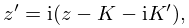
§30.14(iv) Separation of Variables
►The wave equation (30.13.7), transformed to oblate spheroidal coordinates , admits solutions of the form (30.13.8), where satisfies the differential equation …Equation (30.14.7) can be transformed to equation (30.2.1) by the substitution . …33: 15.11 Riemann’s Differential Equation
…
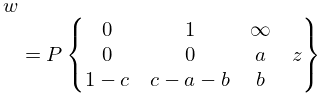
►The importance of (15.10.1) is that any homogeneous linear differential equation of the second order with at most three distinct singularities, all regular, in the extended plane can be transformed into (15.10.1).
…
►
15.11.3
…
►
15.11.4
…
►
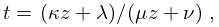
§15.11(ii) Transformation Formulas
… ►
15.11.5
…
34: Errata
35: 21.9 Integrable Equations
…
►Here and are spatial variables, is time, and is the elevation of the surface wave.
All quantities are made dimensionless by a suitable scaling transformation.
…
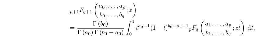
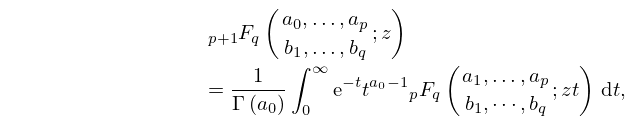
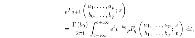
36: 16.5 Integral Representations and Integrals
37: Bibliography T
…
►
LSFBTR: A subroutine for calculating spherical Bessel transforms.
Comput. Phys. Comm. 30 (1), pp. 93–99.
…
►
Laplace type integrals: Transformation to standard form and uniform asymptotic expansions.
Quart. Appl. Math. 43 (1), pp. 103–123.
…
►
Asymptotic expansions of Kummer hypergeometric functions for large values of the parameters.
Integral Transforms Spec. Funct. 33 (1), pp. 16–31.
…
►
A note on the real zeros of the incomplete gamma function.
Integral Transforms Spec. Funct. 23 (6), pp. 445–453.
…
►
Algebraic transformations of hypergeometric functions and automorphic forms on Shimura curves.
Trans. Amer. Math. Soc. 365 (12), pp. 6697–6729.
…
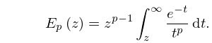
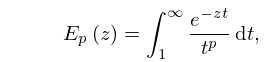
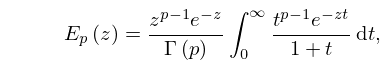
38: 8.19 Generalized Exponential Integral
39: 10.46 Generalized and Incomplete Bessel Functions; Mittag-Leffler Function
…
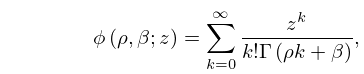
►
10.46.1
.
…
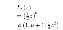
►
10.46.2
…
►The Laplace transform of can be expressed in terms of the Mittag-Leffler function:
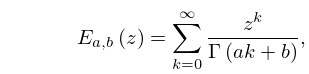
►
10.46.3
.
…
