small k,k′

SearchAdvancedHelp

(0.007 seconds)

21—30 of 70 matching pages

21: 11.13 Methods of Computation

… ►The solution ${𝐊}_{\nu }\left(x\right)$ needs to be integrated backwards for small $x$, and either forwards or backwards for large $x$ depending whether or not $\nu$ exceeds $\frac{1}{2}$. …

22: 22.20 Methods of Computation

… ►By application of the transformations given in §§22.7(i) and 22.7(ii), $k$ or $k^{\prime }$ can always be made sufficently small to enable the approximations given in §22.10(ii) to be applied. …

23: 10.75 Tables

… ►

British Association for the Advancement of Science (1937) tabulates $I_0\left(x\right)$, $I_1\left(x\right)$, $x=0(.001)5$, 7–8D; $K_0\left(x\right)$, $K_1\left(x\right)$, $x=0.01(.01)5$, 7–10D; ${\mathrm{e}}^{-x}{I}_0\left(x\right)$, ${\mathrm{e}}^{-x}{I}_1\left(x\right)$, ${\mathrm{e}}^x{K}_0\left(x\right)$, ${\mathrm{e}}^x{K}_1\left(x\right)$, $x=5(.01)10(.1)20$, 8D. Also included are auxiliary functions to facilitate interpolation of the tables of $K_0\left(x\right)$, $K_1\left(x\right)$ for small values of $x$.

…

24: 36.12 Uniform Approximation of Integrals

… ►For example, the diffraction catastrophe ${\mathrm{\Psi }}_2(x,y;k)$ defined by (36.2.10), and corresponding to the Pearcey integral (36.2.14), can be approximated by the Airy function ${\mathrm{\Psi }}_1\left(\xi (x,y;k)\right)$ when $k$ is large, provided that $x$ and $y$ are not small. …

25: 10.74 Methods of Computation

… ►The power-series expansions given in §§10.2 and 10.8, together with the connection formulas of §10.4, can be used to compute the Bessel and Hankel functions when the argument $x$ or $z$ is sufficiently small in absolute value. In the case of the modified Bessel function $K_{\nu }\left(z\right)$ see especially Temme (1975). … ►It should be noted, however, that there is a difficulty in evaluating the coefficients $A_k(\zeta )$, $B_k(\zeta )$, $C_k(\zeta )$, and $D_k(\zeta )$, from the explicit expressions (10.20.10)–(10.20.13) when $z$ is close to $1$ owing to severe cancellation. … ►For applications of generalized Gauss–Laguerre quadrature (§3.5(v)) to the evaluation of the modified Bessel functions $K_{\nu }\left(z\right)$ for and see Gautschi (2002a). … ►For evaluation of $K_{\nu }\left(z\right)$ from (10.32.14) with $\nu =n$ and $z$ complex, see Mechel (1966). …

26: 9.1 Special Notation

… ► ►►►

$k$	nonnegative integer, except in §9.9(iii).
…
$\delta$	arbitrary small positive constant.
…

…

27: 18.25 Wilson Class: Definitions

… ►

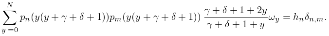
18.25.9 $$\sum _{y=0}^N{p}_n(y(y+\gamma +\delta +1))p_m(y(y+\gamma +\delta +1))\frac{\gamma +\delta +1+2y}{\gamma +\delta +1+y}{\omega }_y=h_n{\delta }_{n,m}.$$

ⓘ

Symbols:

${\delta }_{j,k}$: Kronecker delta, $y$: real variable, $N$: positive integer, $\delta$: arbitrary small positive constant, $p_n(x)$: polynomial of degree $n$ , $m$: nonnegative integer, $n$: nonnegative integer and $h_n$

Referenced by:

§18.38(iii)

Permalink:

http://dlmf.nist.gov/18.25.E9

Encodings:

pMML, png, TeX

See also:

Annotations for §18.25(iii), §18.25 and Ch.18

…

28: 3.5 Quadrature

… ►In particular, when $k=\mathrm{\infty }$ the error term is an exponentially-small function of $1/h$, and in these circumstances the composite trapezoidal rule is exceptionally efficient. …

29: 16.11 Asymptotic Expansions

… ►

$c_k=-{\displaystyle \frac{1}{k{\kappa }^{\kappa }}}{\displaystyle \sum _{m=0}^{k-1}}{c}_m{e}_{k,m},$ $k\ge 1$,

… ►Explicit representations for the coefficients $c_k$ are given in Volkmer (2023). … ►(Either sign may be used when $\mathrm{ph}z=0$ since the first term on the right-hand side becomes exponentially small compared with the second term.) ►Explicit representations for the coefficients $c_k$ are given in Volkmer and Wood (2014). … ►Here $k$ can have any integer value from $1$ to $p$. …

30: 10.45 Functions of Imaginary Order

… ►In consequence of (10.45.5)–(10.45.7), ${\tilde{I}}_{\nu }\left(x\right)$ and ${\tilde{K}}_{\nu }\left(x\right)$ comprise a numerically satisfactory pair of solutions of (10.45.1) when $x$ is large, and either ${\tilde{I}}_{\nu }\left(x\right)$ and $(1/\pi )\sinh \left(\pi \nu \right){\tilde{K}}_{\nu }\left(x\right)$, or ${\tilde{I}}_{\nu }\left(x\right)$ and ${\tilde{K}}_{\nu }\left(x\right)$, comprise a numerically satisfactory pair when $x$ is small, depending whether $\nu \ne 0$ or $\nu =0$. …