small eta

SearchAdvancedHelp

(0.002 seconds)

1—10 of 12 matching pages

1: 33.5 Limiting Forms for Small $\rho$, Small $|\eta |$, or Large $\mathrm{\ell }$

§33.5 Limiting Forms for Small $\rho$, Small $|\eta |$, or Large $\mathrm{\ell }$

►

§33.5(i) Small $\rho$

… ►

§33.5(iii) Small $|\eta |$

…

2: 10.41 Asymptotic Expansions for Large Order

… ►

10.41.12 $$I_{\nu }\left(\nu z\right)=\frac{{\mathrm{e}}^{\nu \eta }}{{(2\pi \nu )}^{\frac{1}{2}}{(1+z^2)}^{\frac{1}{4}}}\left(\sum _{k=0}^{\mathrm{\ell }-1}\frac{U_k(p)}{{\nu }^k}+O\left(\frac{1}{z^{\mathrm{\ell }}}\right)\right),$$ $|\mathrm{ph}z|\le \frac{1}{2}\pi -\delta$,

ⓘ

Symbols:

$O\left(x\right)$: order not exceeding, $\pi$: the ratio of the circumference of a circle to its diameter, $\mathrm{e}$: base of natural logarithm, $I_{\nu }\left(z\right)$: modified Bessel function of the first kind, $\mathrm{ph}$: phase, $k$: nonnegative integer, $z$: complex variable, $\nu$: complex parameter, $\delta$: small positive constant, $\eta$ , $p$ and $U_k(p)$: polynomial coefficient

Referenced by:

§10.41(iv)

Permalink:

http://dlmf.nist.gov/10.41.E12

Encodings:

pMML, png, TeX

See also:

Annotations for §10.41(iv), §10.41 and Ch.10

►

10.41.13 $$K_{\nu }\left(\nu z\right)={\left(\frac{\pi }{2\nu }\right)}^{\frac{1}{2}}\frac{{\mathrm{e}}^{-\nu \eta }}{{(1+z^2)}^{\frac{1}{4}}}\left(\sum _{k=0}^{\mathrm{\ell }-1}{(-1)}^k\frac{U_k(p)}{{\nu }^k}+O\left(\frac{1}{z^{\mathrm{\ell }}}\right)\right),$$ $|\mathrm{ph}z|\le \frac{3}{2}\pi -\delta$.

ⓘ

Symbols:

$O\left(x\right)$: order not exceeding, $\pi$: the ratio of the circumference of a circle to its diameter, $\mathrm{e}$: base of natural logarithm, $K_{\nu }\left(z\right)$: modified Bessel function of the second kind, $\mathrm{ph}$: phase, $k$: nonnegative integer, $z$: complex variable, $\nu$: complex parameter, $\delta$: small positive constant, $\eta$ , $p$ and $U_k(p)$: polynomial coefficient

Referenced by:

§10.41(iv), §10.41(iv)

Permalink:

http://dlmf.nist.gov/10.41.E13

Encodings:

pMML, png, TeX

See also:

Annotations for §10.41(iv), §10.41 and Ch.10

…

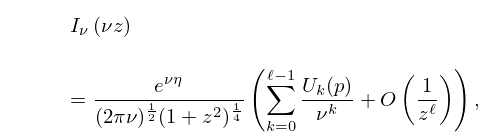
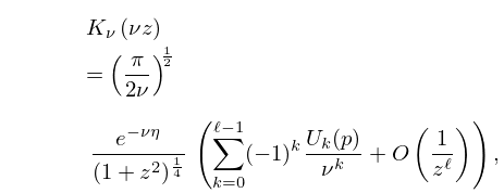
3: 8.12 Uniform Asymptotic Expansions for Large Parameter

… ►

8.12.15 $$Q(a,a)\sim \frac{1}{2}+\frac{1}{\sqrt{2\pi a}}\sum _{k=0}^{\mathrm{\infty }}{c}_k(0)a^{-k},$$ $|\mathrm{ph}a|\le \pi -\delta$,

ⓘ

Symbols:

$\sim$: Poincaré asymptotic expansion, $\pi$: the ratio of the circumference of a circle to its diameter, $Q(a,z)$: normalized incomplete gamma function, $\mathrm{ph}$: phase, $a$: parameter, $k$: nonnegative integer, $\delta$: small positive constant and $c_k(\eta )$: coefficients

Permalink:

http://dlmf.nist.gov/8.12.E15

Encodings:

pMML, png, TeX

See also:

Annotations for §8.12 and Ch.8

►

8.12.16 $$\frac{{\mathrm{e}}^{\pm \pi \mathrm{i}a}}{2\mathrm{i}\sin \left(\pi a\right)}Q(-a,a{\mathrm{e}}^{\pm \pi \mathrm{i}})\sim \pm \frac{1}{2}-\frac{\mathrm{i}}{\sqrt{2\pi a}}\sum _{k=0}^{\mathrm{\infty }}{c}_k(0){(-a)}^{-k},$$ $|\mathrm{ph}a|\le \pi -\delta$,

ⓘ

Symbols:

$\sim$: Poincaré asymptotic expansion, $\pi$: the ratio of the circumference of a circle to its diameter, $\mathrm{e}$: base of natural logarithm, $\mathrm{i}$: imaginary unit, $Q(a,z)$: normalized incomplete gamma function, $\mathrm{ph}$: phase, $\sin z$: sine function, $a$: parameter, $k$: nonnegative integer, $\delta$: small positive constant and $c_k(\eta )$: coefficients

Referenced by:

(8.12.5), Erratum (V1.0.16) for Equation (8.12.5)

Permalink:

http://dlmf.nist.gov/8.12.E16

Encodings:

pMML, png, TeX

See also:

Annotations for §8.12 and Ch.8

…

4: 33.12 Asymptotic Expansions for Large $\eta$

§33.12 Asymptotic Expansions for Large $\eta$

►

§33.12(i) Transition Region

… ►Then as $\eta \to \mathrm{\infty }$, … ►

§33.12(ii) Uniform Expansions

… ►

5: 8.18 Asymptotic Expansions of $I_x(a,b)$

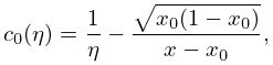
… ►uniformly for $x\in (0,1)$ and $a/(a+b)$, $b/(a+b)\in [\delta ,1-\delta ]$, where $\delta$ again denotes an arbitrary small positive constant. …with $\eta /(x-x_0)>0$, and ►

8.18.11 $$c_0(\eta )=\frac{1}{\eta }-\frac{\sqrt{x_0(1-x_0)}}{x-x_0},$$

ⓘ

Symbols:

$x$: variable and $c_k(\eta )$: coefficients

Permalink:

http://dlmf.nist.gov/8.18.E11

Encodings:

pMML, png, TeX

See also:

Annotations for §8.18(ii), §8.18(ii), §8.18 and Ch.8

… ►For this result, and for higher coefficients $c_k(\eta )$ see Temme (1996b, §11.3.3.2). All of the $c_k(\eta )$ are analytic at $\eta =0$. …

6: 33.23 Methods of Computation

§33.23 Methods of Computation

… ►Thus the regular solutions can be computed from the power-series expansions (§§33.6, 33.19) for small values of the radii and then integrated in the direction of increasing values of the radii. … ►Bardin et al. (1972) describes ten different methods for the calculation of $F_{\mathrm{\ell }}$ and $G_{\mathrm{\ell }}$, valid in different regions of the ($\eta ,\rho$)-plane. … ►Noble (2004) obtains double-precision accuracy for $W_{-\eta ,\mu }\left(2\rho \right)$ for a wide range of parameters using a combination of recurrence techniques, power-series expansions, and numerical quadrature; compare (33.2.7). ►

§33.23(vii) WKBJ Approximations

…

7: 10.75 Tables

… ►

British Association for the Advancement of Science (1937) tabulates $J_0\left(x\right)$, $J_1\left(x\right)$, $x=0(.001)16(.01)25$, 10D; $Y_0\left(x\right)$, $Y_1\left(x\right)$, $x=0.01(.01)25$, 8–9S or 8D. Also included are auxiliary functions to facilitate interpolation of the tables of $Y_0\left(x\right)$, $Y_1\left(x\right)$ for small values of $x$, as well as auxiliary functions to compute all four functions for large values of $x$.

… ►

British Association for the Advancement of Science (1937) tabulates $I_0\left(x\right)$, $I_1\left(x\right)$, $x=0(.001)5$, 7–8D; $K_0\left(x\right)$, $K_1\left(x\right)$, $x=0.01(.01)5$, 7–10D; ${\mathrm{e}}^{-x}{I}_0\left(x\right)$, ${\mathrm{e}}^{-x}{I}_1\left(x\right)$, ${\mathrm{e}}^x{K}_0\left(x\right)$, ${\mathrm{e}}^x{K}_1\left(x\right)$, $x=5(.01)10(.1)20$, 8D. Also included are auxiliary functions to facilitate interpolation of the tables of $K_0\left(x\right)$, $K_1\left(x\right)$ for small values of $x$.

… ►

Olver (1962) provides tables for the uniform asymptotic expansions given in §10.41(ii), including $\eta$ and the coefficients $U_k(p)$, $V_k(p)$ as functions of $p={(1+x^2)}^{-\frac{1}{2}}$. These enable $I_{\nu }\left(\nu x\right)$, $K_{\nu }\left(\nu x\right)$, $I_{\nu }^{\prime }\left(\nu x\right)$, $K_{\nu }^{\prime }\left(\nu x\right)$ to be computed to 10S when $\nu \ge 16$.

… ►

Young and Kirk (1964) tabulates ${\mathrm{ber}}_{n}x$, ${\mathrm{bei}}_{n}x$, ${\ker }_{n}x$, ${\mathrm{kei}}_{n}x$, $n=0,1$, $x=0(.1)10$, 15D; ${\mathrm{ber}}_{n}x$, ${\mathrm{bei}}_{n}x$, ${\ker }_{n}x$, ${\mathrm{kei}}_{n}x$, modulus and phase functions $M_n\left(x\right)$, ${\theta }_n\left(x\right)$, $N_n\left(x\right)$, ${\varphi }_n\left(x\right)$, $n=0,1,2$, $x=0(.01)2.5$, 8S, and $n=0(1)10$, $x=0(.1)10$, 7S. Also included are auxiliary functions to facilitate interpolation of the tables for $n=0(1)10$ for small values of $x$. (Concerning the phase functions see §10.68(iv).)

…

8: 23.22 Methods of Computation

… ►The modular functions $\lambda \left(\tau \right)$, $J\left(\tau \right)$, and $\eta \left(\tau \right)$ are also obtainable in a similar manner from their definitions in §23.15(ii). … ►For $2{\omega }_3$ choose a nonzero point that is not a multiple of $2{\omega }_1$ and is such that $\mathrm{\Im }\tau >0$ and $|\tau |$ is as small as possible, where $\tau ={\omega }_3/{\omega }_1$. …

9: 28.33 Physical Applications

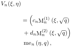
… ►with $W(x,y,t)={\mathrm{e}}^{\mathrm{i}\omega t}V(x,y)$, reduces to (28.32.2) with $k^2={\omega }^2\rho /\tau$. …The separated solutions $V_n(\xi ,\eta )$ must be $2\pi$-periodic in $\eta$, and have the form ►

28.33.2 $$V_n(\xi ,\eta )=\left(c_n{\mathrm{M}}_n^{(1)}(\xi ,\sqrt{q})+d_n{\mathrm{M}}_n^{(2)}(\xi ,\sqrt{q})\right){\mathrm{me}}_n(\eta ,q),$$

ⓘ

Symbols:

${\mathrm{me}}_n(z,q)$: Mathieu function, ${\mathrm{M}}_{\nu }^{(j)}(z,h)$: modified Mathieu function, $q=h^2$: parameter, $n$: integer, $V(\xi ,\eta )$: solution, $d_n$: constants, $\eta$: variable, $\xi$: variable and $c_n$: constants

Permalink:

http://dlmf.nist.gov/28.33.E2

Encodings:

pMML, png, TeX

See also:

Annotations for §28.33(ii), §28.33 and Ch.28

… ►However, in response to a small perturbation at least one solution may become unbounded. …

10: 2.4 Contour Integrals

… ► … ►

2.4.3 $$q(t)=\frac{1}{2\pi \mathrm{i}}\underset{\eta \to \mathrm{\infty }}{lim}{\int }_{\sigma -\mathrm{i}\eta }^{\sigma +\mathrm{i}\eta }{\mathrm{e}}^{tz}Q(z)dz,$$ ,

ⓘ

Symbols:

$\pi$: the ratio of the circumference of a circle to its diameter, $dx$: differential of $x$ , $\mathrm{e}$: base of natural logarithm, $\mathrm{i}$: imaginary unit, $\int$: integral, $q(t)$: analytic function, $Q(z)$: Laplace transform of $q(t)$ and $\sigma$: constant

Referenced by:

§2.4(ii)

Permalink:

http://dlmf.nist.gov/2.4.E3

Encodings:

pMML, png, TeX

See also:

Annotations for §2.4(ii), §2.4 and Ch.2

… ►

2.4.6 $$f(t)=\frac{1}{2\pi \mathrm{i}}\underset{\eta \to \mathrm{\infty }}{lim}{\int }_{\sigma -\mathrm{i}\eta }^{\sigma +\mathrm{i}\eta }{\mathrm{e}}^{tz}F(z)dz$$

ⓘ

Symbols:

$\pi$: the ratio of the circumference of a circle to its diameter, $dx$: differential of $x$ , $\mathrm{e}$: base of natural logarithm, $\mathrm{i}$: imaginary unit, $\int$: integral, $\sigma$: constant, $F(z)$: comparison function and $f(x)$: inverse transform of comparison function

Permalink:

http://dlmf.nist.gov/2.4.E6

Encodings:

pMML, png, TeX

See also:

Annotations for §2.4(ii), §2.4 and Ch.2

… ►

2.4.7 $$q(t)-f(t)=\frac{{\mathrm{e}}^{\sigma t}}{2\pi }\underset{\eta \to \mathrm{\infty }}{lim}{\int }_{-\eta }^{\eta }{\mathrm{e}}^{\mathrm{i}t\tau }(Q(\sigma +\mathrm{i}\tau )-F(\sigma +\mathrm{i}\tau ))d\tau .$$

ⓘ

Symbols:

$\pi$: the ratio of the circumference of a circle to its diameter, $dx$: differential of $x$ , $\mathrm{e}$: base of natural logarithm, $\mathrm{i}$: imaginary unit, $\int$: integral, $q(t)$: analytic function, $Q(z)$: Laplace transform of $q(t)$ , $\sigma$: constant, $F(z)$: comparison function and $f(x)$: inverse transform of comparison function

Permalink:

http://dlmf.nist.gov/2.4.E7

Encodings:

pMML, png, TeX

See also:

Annotations for §2.4(ii), §2.4 and Ch.2

…