sine integrals

SearchAdvancedHelp

(0.010 seconds)

21—30 of 174 matching pages

21: 6.12 Asymptotic Expansions

… ►For the function $\chi$ see §9.7(i). … ►The asymptotic expansions of $\mathrm{Si}\left(z\right)$ and $\mathrm{Ci}\left(z\right)$ are given by (6.2.19), (6.2.20), together with ►

6.12.3 $$\mathrm{f}\left(z\right)\sim \frac{1}{z}\left(1-\frac{2!}{z^2}+\frac{4!}{z^4}-\frac{6!}{z^6}+\mathrm{\cdots }\right),$$

ⓘ

Symbols:

$\sim$: Poincaré asymptotic expansion, $!$: factorial (as in $n!$), $\mathrm{f}\left(z\right)$: auxiliary function for sine and cosine integrals and $z$: complex variable

A&S Ref:

5.2.34

Referenced by:

§6.12(ii), §6.12(ii)

Permalink:

http://dlmf.nist.gov/6.12.E3

Encodings:

pMML, png, TeX

See also:

Annotations for §6.12(ii), §6.12 and Ch.6

►

6.12.4 $$\mathrm{g}\left(z\right)\sim \frac{1}{z^2}\left(1-\frac{3!}{z^2}+\frac{5!}{z^4}-\frac{7!}{z^6}+\mathrm{\cdots }\right),$$

ⓘ

Symbols:

$\sim$: Poincaré asymptotic expansion, $!$: factorial (as in $n!$), $\mathrm{g}\left(z\right)$: auxiliary function for sine and cosine integrals and $z$: complex variable

A&S Ref:

5.2.35

Referenced by:

§6.12(ii), §6.12(ii)

Permalink:

http://dlmf.nist.gov/6.12.E4

Encodings:

pMML, png, TeX

See also:

Annotations for §6.12(ii), §6.12 and Ch.6

… ►

6.12.5 $$\mathrm{f}\left(z\right)=\frac{1}{z}\sum _{m=0}^{n-1}{(-1)}^m\frac{(2m)!}{z^{2m}}+R_n^{(\mathrm{f})}(z),$$

ⓘ

Symbols:

$!$: factorial (as in $n!$), $\mathrm{f}\left(z\right)$: auxiliary function for sine and cosine integrals, $z$: complex variable, $n$: nonnegative integer and $R_n^{(\mathrm{f})}(z)$: remainder term

Referenced by:

§6.12(ii)

Permalink:

http://dlmf.nist.gov/6.12.E5

Encodings:

pMML, png, TeX

See also:

Annotations for §6.12(ii), §6.12 and Ch.6

…

22: 6.17 Physical Applications

§6.17 Physical Applications

… ►Lebedev (1965) gives an application to electromagnetic theory (radiation of a linear half-wave oscillator), in which sine and cosine integrals are used.

23: 7.1 Special Notation

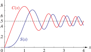
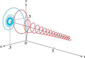
… ►The main functions treated in this chapter are the error function $\mathrm{erf}z$; the complementary error functions $\mathrm{erfc}z$ and $w\left(z\right)$; Dawson’s integral $F\left(z\right)$; the Fresnel integrals $ℱ\left(z\right)$, $C\left(z\right)$, and $S\left(z\right)$; the Goodwin–Staton integral $G\left(z\right)$; the repeated integrals of the complementary error function ${\mathrm{i}}^n\mathrm{erfc}\left(z\right)$; the Voigt functions $𝖴(x,t)$ and $𝖵(x,t)$. ►Alternative notations are $Q(z)=\frac{1}{2}\mathrm{erfc}\left(z/\sqrt{2}\right)$, $P(z)=\mathrm{\Phi }(z)=\frac{1}{2}\mathrm{erfc}\left(-z/\sqrt{2}\right)$, $\mathrm{Erf}z=\frac{1}{2}\sqrt{\pi }\mathrm{erf}z$, $\mathrm{Erfi}z={\mathrm{e}}^{z^2}F\left(z\right)$, $C_1(z)=C\left(\sqrt{2/\pi }z\right)$, $S_1(z)=S\left(\sqrt{2/\pi }z\right)$, $C_2(z)=C\left(\sqrt{2z/\pi }\right)$, $S_2(z)=S\left(\sqrt{2z/\pi }\right)$. …

24: 7.3 Graphics

… ►

►►

Figure 7.3.3: Fresnel integrals $C\left(x\right)$ and $S\left(x\right)$, $0\le x\le 4$. Magnify

…

25: 7.20 Mathematical Applications

… ►Let the set $\{x(t),y(t),t\}$ be defined by $x(t)=C\left(t\right)$, $y(t)=S\left(t\right)$, $t\ge 0$. … ►

►►

Figure 7.20.1: Cornu’s spiral, formed from Fresnel integrals, is defined parametrically by $x=C\left(t\right)$, $y=S\left(t\right)$, $t\in [0,\mathrm{\infty })$. Magnify

…

26: 6.16 Mathematical Applications

… ►

§6.16(i) The Gibbs Phenomenon

… ►

6.16.2 $$S_n(x)=\sum _{k=0}^{n-1}\frac{\sin \left((2k+1)x\right)}{2k+1}=\frac{1}{2}{\int }_0^x\frac{\sin \left(2nt\right)}{\sin t}dt=\frac{1}{2}\mathrm{Si}\left(2nx\right)+R_n(x),$$

ⓘ

Defines:

$S_n(x)$: partial sum (locally)

Symbols:

$dx$: differential of $x$ , $\int$: integral, $\sin z$: sine function, $\mathrm{Si}\left(z\right)$: sine integral, $x$: real variable, $n$: nonnegative integer and $R_n(x)$: remainder term

Permalink:

http://dlmf.nist.gov/6.16.E2

Encodings:

pMML, png, TeX

See also:

Annotations for §6.16(i), §6.16 and Ch.6

… ►

6.16.3 $$R_n(x)=\frac{1}{2}{\int }_0^x\left(\frac{1}{\sin t}-\frac{1}{t}\right)\sin \left(2nt\right)dt.$$

ⓘ

Defines:

$R_n(x)$: remainder term (locally)

Symbols:

$dx$: differential of $x$ , $\int$: integral, $\sin z$: sine function, $x$: real variable and $n$: nonnegative integer

Permalink:

http://dlmf.nist.gov/6.16.E3

Encodings:

pMML, png, TeX

See also:

Annotations for §6.16(i), §6.16 and Ch.6

… ►Hence, if $x$ is fixed and $n\to \mathrm{\infty }$, then $S_n(x)\to \frac{1}{4}\pi$, $0$, or $-\frac{1}{4}\pi$ according as , $x=0$, or ; compare (6.2.14). … ►The first maximum of $\frac{1}{2}\mathrm{Si}\left(x\right)$ for positive $x$ occurs at $x=\pi$ and equals $(1.1789\mathrm{\dots })\times \frac{1}{4}\pi$; compare Figure 6.3.2. …

27: 6.6 Power Series

§6.6 Power Series

… ►

6.6.5 $$\mathrm{Si}\left(z\right)=\sum _{n=0}^{\mathrm{\infty }}\frac{{(-1)}^n{z}^{2n+1}}{(2n+1)!(2n+1)},$$

ⓘ

Symbols:

$!$: factorial (as in $n!$), $\mathrm{Si}\left(z\right)$: sine integral, $z$: complex variable and $n$: nonnegative integer

A&S Ref:

5.2.14

Referenced by:

§6.5

Permalink:

http://dlmf.nist.gov/6.6.E5

Encodings:

pMML, png, TeX

See also:

Annotations for §6.6 and Ch.6

…

28: 10.15 Derivatives with Respect to Order

… ►For the notations $\mathrm{Ci}$ and $\mathrm{Si}$ see §6.2(ii). … ►

10.15.6 $${\frac{\partial J_{\nu }\left(x\right)}{\partial \nu }|}_{\nu =\frac{1}{2}}=\sqrt{\frac{2}{\pi x}}\left(\mathrm{Ci}\left(2x\right)\sin x-\mathrm{Si}\left(2x\right)\cos x\right),$$

ⓘ

Symbols:

$J_{\nu }\left(z\right)$: Bessel function of the first kind, $\pi$: the ratio of the circumference of a circle to its diameter, $\cos z$: cosine function, $\mathrm{Ci}\left(z\right)$: cosine integral, $\frac{\partial f}{\partial x}$: partial derivative of $f$ with respect to $x$ , $\partial x$: partial differential of $x$ , $\sin z$: sine function, $\mathrm{Si}\left(z\right)$: sine integral, $x$: real variable and $\nu$: complex parameter

A&S Ref:

10.1.41 (corrected)

Referenced by:

§10.15, §10.38, Ch.10

Permalink:

http://dlmf.nist.gov/10.15.E6

Encodings:

pMML, png, TeX

See also:

Annotations for §10.15, §10.15 and Ch.10

►

10.15.7 $${\frac{\partial J_{\nu }\left(x\right)}{\partial \nu }|}_{\nu =-\frac{1}{2}}=\sqrt{\frac{2}{\pi x}}\left(\mathrm{Ci}\left(2x\right)\cos x+\mathrm{Si}\left(2x\right)\sin x\right),$$

ⓘ

Symbols:

$J_{\nu }\left(z\right)$: Bessel function of the first kind, $\pi$: the ratio of the circumference of a circle to its diameter, $\cos z$: cosine function, $\mathrm{Ci}\left(z\right)$: cosine integral, $\frac{\partial f}{\partial x}$: partial derivative of $f$ with respect to $x$ , $\partial x$: partial differential of $x$ , $\sin z$: sine function, $\mathrm{Si}\left(z\right)$: sine integral, $x$: real variable and $\nu$: complex parameter

A&S Ref:

10.1.42 (corrected)

Referenced by:

§10.15, §10.38

Permalink:

http://dlmf.nist.gov/10.15.E7

Encodings:

pMML, png, TeX

See also:

Annotations for §10.15, §10.15 and Ch.10

►

10.15.8 $${\frac{\partial Y_{\nu }\left(x\right)}{\partial \nu }|}_{\nu =\frac{1}{2}}=\sqrt{\frac{2}{\pi x}}\left(\mathrm{Ci}\left(2x\right)\cos x+\left(\mathrm{Si}\left(2x\right)-\pi \right)\sin x\right),$$

ⓘ

Symbols:

$Y_{\nu }\left(z\right)$: Bessel function of the second kind, $\pi$: the ratio of the circumference of a circle to its diameter, $\cos z$: cosine function, $\mathrm{Ci}\left(z\right)$: cosine integral, $\frac{\partial f}{\partial x}$: partial derivative of $f$ with respect to $x$ , $\partial x$: partial differential of $x$ , $\sin z$: sine function, $\mathrm{Si}\left(z\right)$: sine integral, $x$: real variable and $\nu$: complex parameter

A&S Ref:

10.1.43 (corrected)

Referenced by:

§10.15

Permalink:

http://dlmf.nist.gov/10.15.E8

Encodings:

pMML, png, TeX

See also:

Annotations for §10.15, §10.15 and Ch.10

►

10.15.9 $${\frac{\partial Y_{\nu }\left(x\right)}{\partial \nu }|}_{\nu =-\frac{1}{2}}=-\sqrt{\frac{2}{\pi x}}\left(\mathrm{Ci}\left(2x\right)\sin x-\left(\mathrm{Si}\left(2x\right)-\pi \right)\cos x\right).$$

ⓘ

Symbols:

$Y_{\nu }\left(z\right)$: Bessel function of the second kind, $\pi$: the ratio of the circumference of a circle to its diameter, $\cos z$: cosine function, $\mathrm{Ci}\left(z\right)$: cosine integral, $\frac{\partial f}{\partial x}$: partial derivative of $f$ with respect to $x$ , $\partial x$: partial differential of $x$ , $\sin z$: sine function, $\mathrm{Si}\left(z\right)$: sine integral, $x$: real variable and $\nu$: complex parameter

A&S Ref:

10.1.44 (corrected)

Referenced by:

§10.15, Ch.10

Permalink:

http://dlmf.nist.gov/10.15.E9

Encodings:

pMML, png, TeX

See also:

Annotations for §10.15, §10.15 and Ch.10

…

29: 7.23 Tables

… ►

Abramowitz and Stegun (1964, Chapter 7) includes $\mathrm{erf}x$, $(2/\sqrt{\pi }){\mathrm{e}}^{-x^2}$, $x\in [0,2]$, 10D; $(2/\sqrt{\pi }){\mathrm{e}}^{-x^2}$, $x\in [2,10]$, 8S; $x{\mathrm{e}}^{x^2}\mathrm{erfc}x$, $x^{-2}\in [0,0.25]$, 7D; $2^n\mathrm{\Gamma }\left(\frac{1}{2}n+1\right){\mathrm{i}}^n\mathrm{erfc}\left(x\right)$, $n=1(1)6,10,11$, $x\in [0,5]$, 6S; $F\left(x\right)$, $x\in [0,2]$, 10D; $xF\left(x\right)$, $x^{-2}\in [0,0.25]$, 9D; $C\left(x\right)$, $S\left(x\right)$, $x\in [0,5]$, 7D; $\mathrm{f}\left(x\right)$, $\mathrm{g}\left(x\right)$, $x\in [0,1]$, $x^{-1}\in [0,1]$, 15D.

… ►

Zhang and Jin (1996, pp. 637, 639) includes $(2/\sqrt{\pi }){\mathrm{e}}^{-x^2}$, $\mathrm{erf}x$, $x=0(.02)1(.04)3$, 8D; $C\left(x\right)$, $S\left(x\right)$, $x=0(.2)10(2)100(100)500$, 8D.

… ►

Zhang and Jin (1996, p. 642) includes the first 10 zeros of $\mathrm{erf}z$, 9D; the first 25 distinct zeros of $C\left(z\right)$ and $S\left(z\right)$, 8S.

30: 7.6 Series Expansions

… ►

7.6.5 $$C\left(z\right)=\cos \left(\frac{1}{2}\pi z^2\right)\sum _{n=0}^{\mathrm{\infty }}\frac{{(-1)}^n{\pi }^{2n}}{1\cdot 3\mathrm{\cdots }(4n+1)}{z}^{4n+1}+\sin \left(\frac{1}{2}\pi z^2\right)\sum _{n=0}^{\mathrm{\infty }}\frac{{(-1)}^n{\pi }^{2n+1}}{1\cdot 3\mathrm{\cdots }(4n+3)}{z}^{4n+3}.$$

ⓘ

Symbols:

$C\left(z\right)$: Fresnel integral, $\pi$: the ratio of the circumference of a circle to its diameter, $\cos z$: cosine function, $\sin z$: sine function, $z$: complex variable and $n$: nonnegative integer

A&S Ref:

7.3.12

Referenced by:

§11.10(vi), §7.6(i)

Permalink:

http://dlmf.nist.gov/7.6.E5

Encodings:

pMML, png, TeX

See also:

Annotations for §7.6(i), §7.6 and Ch.7

►

7.6.6 $$S\left(z\right)=\sum _{n=0}^{\mathrm{\infty }}\frac{{(-1)}^n{(\frac{1}{2}\pi )}^{2n+1}}{(2n+1)!(4n+3)}{z}^{4n+3},$$

ⓘ

Symbols:

$S\left(z\right)$: Fresnel integral, $\pi$: the ratio of the circumference of a circle to its diameter, $!$: factorial (as in $n!$), $z$: complex variable and $n$: nonnegative integer

A&S Ref:

7.3.13

Referenced by:

§7.6(i)

Permalink:

http://dlmf.nist.gov/7.6.E6

Encodings:

pMML, png, TeX

See also:

Annotations for §7.6(i), §7.6 and Ch.7

►

7.6.7 $$S\left(z\right)=-\cos \left(\frac{1}{2}\pi z^2\right)\sum _{n=0}^{\mathrm{\infty }}\frac{{(-1)}^n{\pi }^{2n+1}}{1\cdot 3\mathrm{\cdots }(4n+3)}{z}^{4n+3}+\sin \left(\frac{1}{2}\pi z^2\right)\sum _{n=0}^{\mathrm{\infty }}\frac{{(-1)}^n{\pi }^{2n}}{1\cdot 3\mathrm{\cdots }(4n+1)}{z}^{4n+1}.$$

ⓘ

Symbols:

$S\left(z\right)$: Fresnel integral, $\pi$: the ratio of the circumference of a circle to its diameter, $\cos z$: cosine function, $\sin z$: sine function, $z$: complex variable and $n$: nonnegative integer

A&S Ref:

7.3.14

Referenced by:

§11.10(vi), §7.6(i)

Permalink:

http://dlmf.nist.gov/7.6.E7

Encodings:

pMML, png, TeX

See also:

Annotations for §7.6(i), §7.6 and Ch.7

… ►

7.6.11 $$S\left(z\right)=z\sum _{n=0}^{\mathrm{\infty }}{𝗃}_{2n+1}\left(\frac{1}{2}\pi z^2\right).$$

ⓘ

Symbols:

$S\left(z\right)$: Fresnel integral, $\pi$: the ratio of the circumference of a circle to its diameter, ${𝗃}_n\left(z\right)$: spherical Bessel function of the first kind, $z$: complex variable and $n$: nonnegative integer

Referenced by:

§7.6(ii)

Permalink:

http://dlmf.nist.gov/7.6.E11

Encodings:

pMML, png, TeX

See also:

Annotations for §7.6(ii), §7.6 and Ch.7

…