simple
(0.001 seconds)
21—30 of 72 matching pages
21: 1.6 Vectors and Vector-Valued Functions
…
►The geometrical image of a path is called a simple
closed curve if is one-to-one, with the exception .
…
…
►and be the closed and bounded point set in the plane having a simple closed curve as boundary.
…
22: 3.3 Interpolation
…
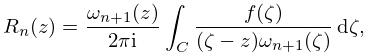
►
3.3.6
►where is a simple closed contour in described in the positive rotational sense and enclosing the points .
…
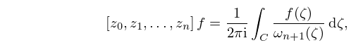
►
3.3.37
►where is given by (3.3.3), and is a simple closed contour in described in the positive rotational sense and enclosing .
…
23: 20.13 Physical Applications
…
►Theta-function solutions to the heat diffusion equation with simple boundary conditions are discussed in Lawden (1989, pp. 1–3), and with more general boundary conditions in Körner (1989, pp. 274–281).
…
24: 28.7 Analytic Continuation of Eigenvalues
25: 2.8 Differential Equations with a Parameter
…
►In Case II has a simple zero at and is analytic at .
…
►
§2.8(iii) Case II: Simple Turning Point
… ►§2.8(iv) Case III: Simple Pole
… ►More generally, can have a simple or double pole at . … ►For a coalescing turning point and simple pole see Nestor (1984) and Dunster (1994b); in this case the uniform approximants are Whittaker functions (§13.14(i)) with a fixed value of the second parameter. …26: 7.13 Zeros
…
►
has a simple zero at , and in the first quadrant of there is an infinite set of zeros , , arranged in order of increasing absolute value.
…
►At , has a simple zero and has a triple zero.
…
27: 18.40 Methods of Computation
…
►In what follows we consider only the simple, illustrative, case that is continuously differentiable so that , with real, positive, and continuous on a real interval The strategy will be to: 1) use the moments to determine the recursion coefficients of equations (18.2.11_5) and (18.2.11_8); then, 2) to construct the quadrature abscissas and weights (or Christoffel numbers) from the J-matrix of §3.5(vi), equations (3.5.31) and(3.5.32).
…
►A simple set of choices is spelled out in Gordon (1968) which gives a numerically stable algorithm for direct computation of the recursion coefficients in terms of the moments, followed by construction of the J-matrix and quadrature weights and abscissas, and we will follow this approach: Let be a positive integer and define
…
28: 22.2 Definitions
…
►Each is meromorphic in for fixed , with simple poles and simple zeros, and each is meromorphic in for fixed .
…
29: 25.2 Definition and Expansions
…
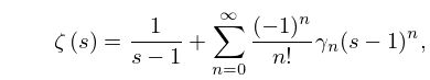
►It is a meromorphic function whose only singularity in is a simple pole at , with residue 1.
…
►
25.2.4
…
