representations as sums of powers
(0.002 seconds)
11—20 of 26 matching pages
11: 27.14 Unrestricted Partitions
…
►A fundamental problem studies the number of ways can be written as a sum of positive integers , that is, the number of solutions of
…
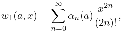
►Multiplying the power series for with that for and equating coefficients, we obtain the recursion formula
…
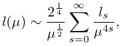
►and is a Dedekind sum given by
…
►where and is given by (27.14.11).
…
►The 24th power of in (27.14.12) with is an infinite product that generates a power series in with integer coefficients called Ramanujan’s tau function
:
…
12: 18.3 Definitions
…
►For representations of the polynomials in Table 18.3.1 by Rodrigues formulas, see §18.5(ii).
For finite power series of the Jacobi, ultraspherical, Laguerre, and Hermite polynomials, see §18.5(iii) (in powers of for Jacobi polynomials, in powers of for the other cases).
Explicit power series for Chebyshev, Legendre, Laguerre, and Hermite polynomials for are given in §18.5(iv).
For explicit power series coefficients up to for these polynomials and for coefficients up to for Jacobi and ultraspherical polynomials see Abramowitz and Stegun (1964, pp. 793–801).
…
►When the sum in (18.3.1) is .
…
13: 12.14 The Function
…
►
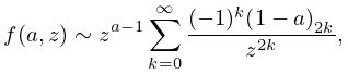
§12.14(v) Power-Series Expansions
… ►
12.14.9
►
12.14.10
…
►
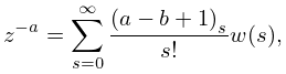
§12.14(vi) Integral Representations
… ►
12.14.29
…
14: 8.21 Generalized Sine and Cosine Integrals
…
►
§8.21(iii) Integral Representations
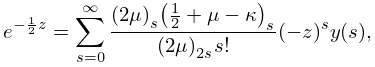
… ►In these representations the integration paths do not cross the negative real axis, and in the case of (8.21.4) and (8.21.5) the paths also exclude the origin. … ►Power-Series Expansions
… ►
8.21.21
…
►
8.21.26
…
15: 13.29 Methods of Computation
…
►A comprehensive and powerful approach is to integrate the differential equations (13.2.1) and (13.14.1) by direct numerical methods.
…
►
§13.29(iii) Integral Representations
►The integral representations (13.4.1) and (13.4.4) can be used to compute the Kummer functions, and (13.16.1) and (13.16.5) for the Whittaker functions. … ►
13.29.3
…
►
13.29.7
…
16: 5.9 Integral Representations
§5.9 Integral Representations
… ►(The fractional powers have their principal values.) … ►For additional representations see Whittaker and Watson (1927, §§12.31–12.32). … ► …17: Bibliography
…
►
Integral representation of Kelvin functions and their derivatives with respect to the order.
Z. Angew. Math. Phys. 42 (5), pp. 708–714.
…
►
Theorems on generalized Dedekind sums.
Pacific J. Math. 2 (1), pp. 1–9.
…
►
Bernoulli’s power-sum formulas revisited.
Math. Gaz. 90 (518), pp. 276–279.
…
►
Integral representations for Jacobi polynomials and some applications.
J. Math. Anal. Appl. 26 (2), pp. 411–437.
…
►
Jacobi polynomials. I. New proofs of Koornwinder’s Laplace type integral representation and Bateman’s bilinear sum.
SIAM J. Math. Anal. 5, pp. 119–124.
…
18: 2.4 Contour Integrals
…
►
(a)
…
►However, if , then and different branches of some of the fractional powers of are used for the coefficients ; again see §2.3(iii).
…
►For integral representations of the and their asymptotic behavior as see Boyd (1995).
…
2.4.1
…
►
2.4.4
,
…
►
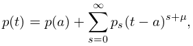
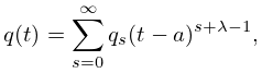
In a neighborhood of
2.4.11
with , , , and the branches of and continuous and constructed with as along .
19: Bibliography G
…
►
Integral representations for computing real parabolic cylinder functions.
Numer. Math. 98 (1), pp. 105–134.
…
►
Stirling number representation problems.
Proc. Amer. Math. Soc. 11 (3), pp. 447–451.
…
►
A monotonicity property of the power function of multivariate tests.
Indag. Math. (N.S.) 11 (2), pp. 209–218.
…
►
Bessel functions and representation theory. I.
J. Functional Analysis 22 (2), pp. 73–105.
…
►
Representations of Integers as Sums of Squares.
Springer-Verlag, New York.
…
20: 19.36 Methods of Computation
…
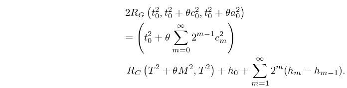
►When the differences are moderately small, the iteration is stopped, the elementary symmetric functions of certain differences are calculated, and a polynomial consisting of a fixed number of terms of the sum in (19.19.7) is evaluated.
…
►
19.36.13
…
►Numerical quadrature is slower than most methods for the standard integrals but can be useful for elliptic integrals that have complicated representations in terms of standard integrals.
…
►Faster convergence of power series for and can be achieved by using (19.5.1) and (19.5.2) in the right-hand sides of (19.8.12).
…
