q-zAl-Salam--Chihara polynomials

SearchAdvancedHelp

(0.003 seconds)

11—20 of 255 matching pages

11: 18.20 Hahn Class: Explicit Representations

… ►

§18.20(i) Rodrigues Formulas

… ►For the Hahn polynomials $p_n(x)=Q_n(x;\alpha ,\beta ,N)$ and …For the Krawtchouk, Meixner, and Charlier polynomials, $F(x)$ and ${\kappa }_n$ are as in Table 18.20.1. … ►

§18.20(ii) Hypergeometric Function and Generalized Hypergeometric Functions

… ►(For symmetry properties of $p_n(x;a,b,\overline{a},\overline{b})$ with respect to $a$, $b$, $\overline{a}$, $\overline{b}$ see Andrews et al. (1999, Corollary 3.3.4).) …

12: Bibliography N

… ►

Orthogonal polynomials. Mem. Amer. Math. Soc. 18 (213), pp. v+185 pp..

ⓘ

External Links:

ISSN 0065-9266, Document, Link, MathReview (T. S. Chihara)

Referenced by:

§18.2(xi), §18.2(xi).

Encodings:

BibTeX

►

Géza Freud, orthogonal polynomials and Christoffel functions. A case study. J. Approx. Theory 48 (1), pp. 3–167.

ⓘ

External Links:

ISSN 0021-9045, Document, MathReview (T. S. Chihara), ZentralBlatt

Referenced by:

§18.32.

Encodings:

BibTeX

… ►

Askey-Wilson polynomials: an affine Hecke algebra approach. In Laredo Lectures on Orthogonal Polynomials and Special Functions, Adv. Theory Spec. Funct. Orthogonal Polynomials, pp. 111–144.

ⓘ

External Links:

MathReview (V. L. Deshpande), ZentralBlatt

Referenced by:

§18.38(iii).

Encodings:

BibTeX

… ►

Symmetries in the fourth Painlevé equation and Okamoto polynomials. Nagoya Math. J. 153, pp. 53–86.

ⓘ

External Links:

ISSN 0027-7630, MathReview (Andrei A. Kapaev), ZentralBlatt

Referenced by:

§32.8(iv).

Encodings:

BibTeX

…

13: Bibliography Z

… ►

Doron Zeilberger’s Maple Packages and Programs Department of Mathematics, Rutgers University, New Jersey.

ⓘ

Notes:

Includes hypergeometric and $q$-hypergeometric summation, solution of difference equations (for example, by Petkovšek’s algorithm), combinatorial algorithms, and (package LUC) evaluation of zonal polynomials.

External Links:

Home Page

Referenced by:

§ ‣ Software Cross Index, § ‣ Software Cross Index, L. Lapointe and L. Vinet (1996).

Encodings:

BibTeX

… ►

Weighted derangements and the linearization coefficients of orthogonal Sheffer polynomials. Proc. London Math. Soc. (3) 65 (1), pp. 1–22.

ⓘ

External Links:

ISSN 0024-6115, Document, Link, MathReview (R. A. Askey), ZentralBlatt

Referenced by:

§18.18(v).

Encodings:

BibTeX

… ►

“Hidden symmetry” of Askey-Wilson polynomials. Theoret. and Math. Phys. 89 (2), pp. 1146–1157.

ⓘ

External Links:

MathReview (Vadim B. Kuznetsov), ZentralBlatt

Referenced by:

§18.38(iii).

Encodings:

BibTeX

►

On some classes of polynomials orthogonal on arcs of the unit circle connected with symmetric orthogonal polynomials on an interval. J. Approx. Theory 94 (1), pp. 73–106.

ⓘ

External Links:

ISSN 0021-9045, Link, MathReview (T. S. Chihara), ZentralBlatt

Referenced by:

§18.33(iii).

Encodings:

BibTeX

…

14: 24.18 Physical Applications

§24.18 Physical Applications

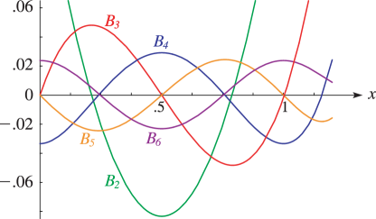
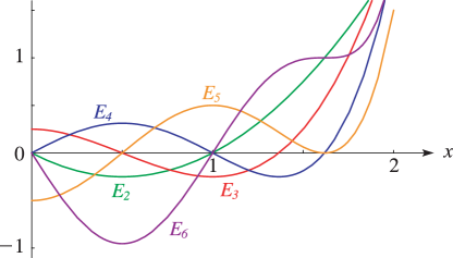
►Bernoulli polynomials appear in statistical physics (Ordóñez and Driebe (1996)), in discussions of Casimir forces (Li et al. (1991)), and in a study of quark-gluon plasma (Meisinger et al. (2002)). ►Euler polynomials also appear in statistical physics as well as in semi-classical approximations to quantum probability distributions (Ballentine and McRae (1998)).

15: Bibliography C

… ►

A note on Euler numbers and polynomials. Nagoya Math. J. 7, pp. 35–43.

ⓘ

External Links:

MathReview (A. L. Whiteman), ZentralBlatt

Referenced by:

§24.10(iv).

Encodings:

BibTeX

… ►

Stability properties of disk polynomials. Numer. Algorithms.

ⓘ

External Links:

Document

Referenced by:

(18.14.3_5).

Encodings:

BibTeX

… ►

On the zeros of the Askey-Wilson polynomials, with applications to coding theory. SIAM J. Math. Anal. 18 (1), pp. 191–207.

ⓘ

External Links:

ISSN 0036-1410, Document, MathReview (Mourad E. H. Ismail), ZentralBlatt

Referenced by:

§18.38(iii).

Encodings:

BibTeX

►

An Introduction to Orthogonal Polynomials. Mathematics and its Applications, Vol. 13, Gordon and Breach Science Publishers, New York.

ⓘ

External Links:

ISBN 0-677-04150-0, MathReview (A. G. Law), ZentralBlatt

Referenced by:

§1.16(ix), (18.2.33), (18.2.36), (18.2.38), §18.2(v), §18.2(iii), §18.2(iv), §18.2(vii), §18.2(x), §18.20(i), (18.30.25), §18.30(ii), §18.30, §18.40(ii), Ch.18.

Encodings:

BibTeX

►

Extremal measures for a system of orthogonal polynomials. Constr. Approx. 9, pp. 111–119.

ⓘ

External Links:

ISSN 0176-4276, Document, MathReview (Mizan Rahman), ZentralBlatt

Referenced by:

§18.28(iv).

Encodings:

BibTeX

…

16: 24.3 Graphs

… ►

►►

Figure 24.3.1: Bernoulli polynomials $B_n\left(x\right)$, $n=2,3,\mathrm{\dots },6$. Magnify

►

►►

Figure 24.3.2: Euler polynomials $E_n\left(x\right)$, $n=2,3,\mathrm{\dots },6$. Magnify

17: 18.4 Graphics

… ►

►►

Figure 18.4.1: Jacobi polynomials $P_n^{(1.5,-0.5)}\left(x\right)$, $n=1,2,3,4,5$. Magnify

►

►►

Figure 18.4.2: Jacobi polynomials $P_n^{(1.25,0.75)}\left(x\right)$, $n=7,8$. … Magnify

… ►

►►

Figure 18.4.4: Legendre polynomials $P_n\left(x\right)$, $n=1,2,3,4,5$. Magnify

►

►►

Figure 18.4.5: Laguerre polynomials $L_n\left(x\right)$, $n=1,2,3,4,5$. Magnify

… ►

►►

Figure 18.4.7: Monic Hermite polynomials $h_n(x)=2^{-n}{H}_n\left(x\right)$, $n=1,2,3,4,5$. Magnify

…

18: 18.7 Interrelations and Limit Relations

§18.7 Interrelations and Limit Relations

… ►

Chebyshev, Ultraspherical, and Jacobi

… ►

Legendre, Ultraspherical, and Jacobi

… ►

§18.7(ii) Quadratic Transformations

… ►

§18.7(iii) Limit Relations

…

19: 18.40 Methods of Computation

… ►

§18.40(i) Computation of Polynomials

►Orthogonal polynomials can be computed from their explicit polynomial form by Horner’s scheme (§1.11(i)). … … ►The theory behind these remarks is in Shohat and Tamarkin (1970), Akhiezer (2021), Chihara (1978). … ►The example chosen is inversion from the ${\alpha }_n,{\beta }_n$ for the weight function for the repulsive Coulomb–Pollaczek, RCP, polynomials of (18.39.50). …

20: 18.41 Tables

… ►

§18.41(i) Polynomials

►For $P_n\left(x\right)$ ($={𝖯}_n\left(x\right)$) see §14.33. ►Abramowitz and Stegun (1964, Tables 22.4, 22.6, 22.11, and 22.13) tabulates $T_n\left(x\right)$, $U_n\left(x\right)$, $L_n\left(x\right)$, and $H_n\left(x\right)$ for $n=0(1)12$. The ranges of $x$ are $0.2(.2)1$ for $T_n\left(x\right)$ and $U_n\left(x\right)$, and $0.5,1,3,5,10$ for $L_n\left(x\right)$ and $H_n\left(x\right)$. … ►For $P_n\left(x\right)$, $L_n\left(x\right)$, and $H_n\left(x\right)$ see §3.5(v). …