principal branch (value)

SearchAdvancedHelp

(0.004 seconds)

31—40 of 102 matching pages

31: 19.2 Definitions

… ►with a branch point at $k=0$ and principal branch $|\mathrm{ph}k|\le \pi$. … ►If , then the integral in (19.2.11) is a Cauchy principal value. … ►where the Cauchy principal value is taken if . … ►In (19.2.18)–(19.2.22) the inverse trigonometric and hyperbolic functions assume their principal values (§§4.23(ii) and 4.37(ii)). …The Cauchy principal value is hyperbolic: …

32: 5.7 Series Expansions

… ►For 15D numerical values of $c_k$ see Abramowitz and Stegun (1964, p. 256), and for 31D values see Wrench (1968). ►

5.7.3 $$\ln \mathrm{\Gamma }\left(1+z\right)=-\ln \left(1+z\right)+z(1-\gamma )+\sum _{k=2}^{\mathrm{\infty }}{(-1)}^k(\zeta \left(k\right)-1)\frac{z^k}{k},$$ .

ⓘ

Symbols:

$\mathrm{\Gamma }\left(z\right)$: gamma function, $\gamma$: Euler’s constant, $\zeta \left(s\right)$: Riemann zeta function, $\ln z$: principal branch of logarithm function, $k$: nonnegative integer and $z$: complex variable

A&S Ref:

6.1.33

Referenced by:

§5.21, §5.7(i)

Permalink:

http://dlmf.nist.gov/5.7.E3

Encodings:

pMML, png, TeX

See also:

Annotations for §5.7(i), §5.7 and Ch.5

… ►For 20D numerical values of the coefficients of the Maclaurin series for $\mathrm{\Gamma }\left(z+3\right)$ see Luke (1969b, p. 299). …

33: 8.17 Incomplete Beta Functions

… ►where and the branches of $s^{-a}$ and ${(1-s)}^{-b}$ are continuous on the path and assume their principal values when $s=c$. …

34: 1.14 Integral Transforms

… ►The Fourier transform of a real- or complex-valued function $f(t)$ is defined by … ►where the last integral denotes the Cauchy principal value (1.4.25). … ►Suppose $f(t)$ is a real- or complex-valued function and $s$ is a real or complex parameter. … ►The Mellin transform of a real- or complex-valued function $f(x)$ is defined by … ►The Stieltjes transform of a real-valued function $f(t)$ is defined by …

35: 14.24 Analytic Continuation

… ►Let $s$ be an arbitrary integer, and $P_{\nu }^{-\mu }\left(z{\mathrm{e}}^{s\pi \mathrm{i}}\right)$ and ${𝑸}_{\nu }^{\mu }\left(z{\mathrm{e}}^{s\pi \mathrm{i}}\right)$ denote the branches obtained from the principal branches by making $\frac{1}{2}s$ circuits, in the positive sense, of the ellipse having $\pm 1$ as foci and passing through $z$. …the limiting value being taken in (14.24.1) when $2\nu$ is an odd integer. ►Next, let $P_{\nu ,s}^{-\mu }\left(z\right)$ and ${𝑸}_{\nu ,s}^{\mu }\left(z\right)$ denote the branches obtained from the principal branches by encircling the branch point $1$ (but not the branch point $-1$) $s$ times in the positive sense. …the limiting value being taken in (14.24.4) when $\mu \in \mathbb{Z}$. ►For fixed $z$, other than $\pm 1$ or $\mathrm{\infty }$, each branch of $P_{\nu }^{-\mu }\left(z\right)$ and ${𝑸}_{\nu }^{\mu }\left(z\right)$ is an entire function of each parameter $\nu$ and $\mu$. …

36: 4.13 Lambert $W$-Function

… ►We call the increasing solution for which $W\left(z\right)\ge W\left(-{\mathrm{e}}^{-1}\right)=-1$ the principal branch and denote it by $W_0\left(z\right)$. … ►Other solutions of (4.13.1) are other branches of $W\left(z\right)$. …$W_0\left(z\right)$ is a single-valued analytic function on $ℂ\setminus (-\mathrm{\infty },-{\mathrm{e}}^{-1}]$, real-valued when $z>-{\mathrm{e}}^{-1}$, and has a square root branch point at $z=-{\mathrm{e}}^{-1}$. …The other branches $W_k\left(z\right)$ are single-valued analytic functions on $ℂ\setminus (-\mathrm{\infty },0]$, have a logarithmic branch point at $z=0$, and, in the case $k=\pm 1$, have a square root branch point at $z=-{\mathrm{e}}^{-1}\mp 0\mathrm{i}$ respectively. … ►where $t\ge 0$ for $W_0$, $t\le 0$ for $W_{\pm 1}$ on the relevant branch cuts, …

37: 25.6 Integer Arguments

… ►

§25.6(i) Function Values

… ►

§25.6(ii) Derivative Values

►

25.6.11 $${\zeta }^{\prime }\left(0\right)=-\frac{1}{2}\ln \left(2\pi \right).$$

ⓘ

Symbols:

$\zeta \left(s\right)$: Riemann zeta function, $\pi$: the ratio of the circumference of a circle to its diameter and $\ln z$: principal branch of logarithm function

Source:

Apostol (1985a, p. 223)

A&S Ref:

23.2.13

Permalink:

http://dlmf.nist.gov/25.6.E11

Encodings:

pMML, png, TeX

See also:

Annotations for §25.6(ii), §25.6 and Ch.25

►

25.6.12 $${\zeta }^{\prime \prime }\left(0\right)=-\frac{1}{2}{(\ln \left(2\pi \right))}^2+\frac{1}{2}{\gamma }^2-\frac{1}{24}{\pi }^2+{\gamma }_1,$$

ⓘ

Symbols:

$\gamma$: Euler’s constant, $\zeta \left(s\right)$: Riemann zeta function, ${\gamma }_n$: Stieltjes constants, $\pi$: the ratio of the circumference of a circle to its diameter and $\ln z$: principal branch of logarithm function

Source:

Apostol (1985a, pp. 226, 227, 229)

Referenced by:

Erratum (V1.0.23) for Subsection 25.2(ii) Other Infinite Series

Permalink:

http://dlmf.nist.gov/25.6.E12

Encodings:

pMML, png, TeX

See also:

Annotations for §25.6(ii), §25.6 and Ch.25

… ►

25.6.15 $${\zeta }^{\prime }\left(2n\right)=\frac{{(-1)}^{n+1}{(2\pi )}^{2n}}{2(2n)!}\left(2n{\zeta }^{\prime }\left(1-2n\right)-(\psi \left(2n\right)-\ln \left(2\pi \right))B_{2n}\right).$$

ⓘ

Symbols:

$B_n$: Bernoulli numbers, $\zeta \left(s\right)$: Riemann zeta function, $\pi$: the ratio of the circumference of a circle to its diameter, $\psi \left(z\right)$: psi (or digamma) function, $!$: factorial (as in $n!$), $\ln z$: principal branch of logarithm function and $n$: nonnegative integer

Source:

Miller and Adamchik (1998, (2), p. 202)

Referenced by:

(25.11.21)

Permalink:

http://dlmf.nist.gov/25.6.E15

Encodings:

pMML, png, TeX

See also:

Annotations for §25.6(ii), §25.6 and Ch.25

…

38: 19.3 Graphics

… ►

►

►

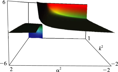
Figure 19.3.5: $\mathrm{\Pi }({\alpha }^2,k)$ as a function of $k^2$ and ${\alpha }^2$ for , $-2\le {\alpha }^2\le 2$. Cauchy principal values are shown when ${\alpha }^2>1$. … Magnify 3D Help

►

►

►

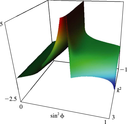
Figure 19.3.6: $\mathrm{\Pi }(\varphi ,2,k)$ as a function of $k^2$ and ${\sin }^2\varphi$ for $-1\le k^2\le 3$, . Cauchy principal values are shown when ${\sin }^2\varphi >\frac{1}{2}$. … Magnify 3D Help

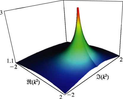
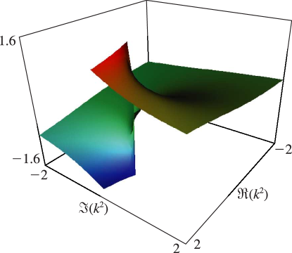
… ►In Figures 19.3.7 and 19.3.8 for complete Legendre’s elliptic integrals with complex arguments, height corresponds to the absolute value of the function and color to the phase. … ►

►

►

Figure 19.3.9: $\mathrm{\Re }\left(K\left(k\right)\right)$ as a function of complex $k^2$ for $-2\le \mathrm{\Re }\left(k^2\right)\le 2$, $-2\le \mathrm{\Im }\left(k^2\right)\le 2$. …On the branch cut ($k^2\ge 1$) it is infinite at $k^2=1$, and has the value $K(1/k)/k$ when $k^2>1$. Magnify 3D Help

►

►

►

Figure 19.3.10: $\mathrm{\Im }\left(K\left(k\right)\right)$ as a function of complex $k^2$ for $-2\le \mathrm{\Re }\left(k^2\right)\le 2$, $-2\le \mathrm{\Im }\left(k^2\right)\le 2$. …On the upper edge of the branch cut ($k^2\ge 1$) it has the value $K\left(k^{\prime }\right)$ if $k^2>1$, and $\frac{1}{4}\pi$ if $k^2=1$. Magnify 3D Help

…

39: 6.6 Power Series

… ►

6.6.1 $$\mathrm{Ei}\left(x\right)=\gamma +\ln x+\sum _{n=1}^{\mathrm{\infty }}\frac{x^n}{n!n},$$ $x>0$.

ⓘ

Symbols:

$\gamma$: Euler’s constant, $\mathrm{Ei}\left(x\right)$: exponential integral, $!$: factorial (as in $n!$), $\ln z$: principal branch of logarithm function, $x$: real variable and $n$: nonnegative integer

A&S Ref:

5.1.10

Referenced by:

§6.5

Permalink:

http://dlmf.nist.gov/6.6.E1

Encodings:

pMML, png, TeX

See also:

Annotations for §6.6 and Ch.6

►

6.6.2 $$E_1\left(z\right)=-\gamma -\ln z-\sum _{n=1}^{\mathrm{\infty }}\frac{{(-1)}^n{z}^n}{n!n}.$$

ⓘ

Symbols:

$\gamma$: Euler’s constant, $E_1\left(z\right)$: exponential integral, $!$: factorial (as in $n!$), $\ln z$: principal branch of logarithm function, $z$: complex variable and $n$: nonnegative integer

A&S Ref:

5.1.11

Referenced by:

§6.4, §6.5

Permalink:

http://dlmf.nist.gov/6.6.E2

Encodings:

pMML, png, TeX

See also:

Annotations for §6.6 and Ch.6

►

6.6.3 $$E_1\left(z\right)=-\ln z+{\mathrm{e}}^{-z}\sum _{n=0}^{\mathrm{\infty }}\frac{z^n}{n!}\psi \left(n+1\right),$$

ⓘ

Symbols:

$\psi \left(z\right)$: psi (or digamma) function, $\mathrm{e}$: base of natural logarithm, $E_1\left(z\right)$: exponential integral, $!$: factorial (as in $n!$), $\ln z$: principal branch of logarithm function, $z$: complex variable and $n$: nonnegative integer

Referenced by:

§2.5(iii), §6.6, §8.19(iv)

Permalink:

http://dlmf.nist.gov/6.6.E3

Encodings:

pMML, png, TeX

See also:

Annotations for §6.6 and Ch.6

… ►

6.6.6 $$\mathrm{Ci}\left(z\right)=\gamma +\ln z+\sum _{n=1}^{\mathrm{\infty }}\frac{{(-1)}^n{z}^{2n}}{(2n)!(2n)}.$$

ⓘ

Symbols:

$\gamma$: Euler’s constant, $\mathrm{Ci}\left(z\right)$: cosine integral, $!$: factorial (as in $n!$), $\ln z$: principal branch of logarithm function, $z$: complex variable and $n$: nonnegative integer

A&S Ref:

5.2.16

Referenced by:

§6.5

Permalink:

http://dlmf.nist.gov/6.6.E6

Encodings:

pMML, png, TeX

See also:

Annotations for §6.6 and Ch.6

►The series in this section converge for all finite values of $x$ and $|z|$.

40: 10.21 Zeros

… ►For the first zeros rounded numerical values of the coefficients are given by … ►This subsection describes the distribution in $ℂ$ of the zeros of the principal branches of the Bessel functions of the second and third kinds, and their derivatives, in the case when the order is a positive integer $n$. For further information, including uniform asymptotic expansions, extensions to other branches of the functions and their derivatives, and extensions to half-integer values of the order, see Olver (1954). … ►The first set of zeros of the principal value of $Y_n\left(nz\right)$ are the points $z=y_{n,m}/n$, $m=1,2,\mathrm{\dots }$, on the positive real axis (§10.21(i)). … ►The first set of zeros of the principal value of $H_n^{(1)}\left(nz\right)$ is an infinite string with asymptote $\mathrm{\Im }z=-\mathrm{i}d/n$, where …