partial

SearchAdvancedHelp

(0.000 seconds)

31—40 of 95 matching pages

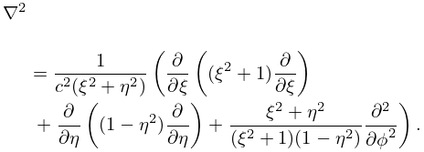
31: 30.14 Wave Equation in Oblate Spheroidal Coordinates

… ►

30.14.6 $${\nabla }^2=\frac{1}{c^2({\xi }^2+{\eta }^2)}\left(\frac{\partial }{\partial \xi }\left(({\xi }^2+1)\frac{\partial }{\partial \xi }\right)+\frac{\partial }{\partial \eta }\left((1-{\eta }^2)\frac{\partial }{\partial \eta }\right)+\frac{{\xi }^2+{\eta }^2}{({\xi }^2+1)(1-{\eta }^2)}\frac{{\partial }^2}{{\partial \varphi }^2}\right).$$

ⓘ

Symbols:

$\frac{\partial f}{\partial x}$: partial derivative of $f$ with respect to $x$ , $\partial x$: partial differential of $x$ , $\xi$: oblate spheroidal coordinate, $\eta$: oblate spheroidal coordinate, $\varphi$: oblate spheroidal coordinate and $c$: positive constant

A&S Ref:

21.5.2 (in corrected form)

Permalink:

http://dlmf.nist.gov/30.14.E6

Encodings:

pMML, png, TeX

See also:

Annotations for §30.14(iii), §30.14 and Ch.30

…

32: 1.9 Calculus of a Complex Variable

… ►

${\displaystyle \frac{\partial u}{\partial x}}={\displaystyle \frac{\partial v}{\partial y}},$

►

${\displaystyle \frac{\partial u}{\partial y}}=-{\displaystyle \frac{\partial v}{\partial x}}$

… ►Conversely, if at a given point $(x,y)$ the partial derivatives $\partial u/\partial x$, $\partial u/\partial y$, $\partial v/\partial x$, and $\partial v/\partial y$ exist, are continuous, and satisfy (1.9.25), then $f(z)$ is differentiable at $z=x+\mathrm{i}y$. … ►

1.9.26 $$\frac{{\partial }^{2}u}{{\partial x}^2}+\frac{{\partial }^{2}u}{{\partial y}^2}=\frac{{\partial }^{2}v}{{\partial x}^2}+\frac{{\partial }^{2}v}{{\partial y}^2}=0,$$

ⓘ

Symbols:

$\frac{\partial f}{\partial x}$: partial derivative of $f$ with respect to $x$ , $\partial x$: partial differential of $x$ , $u(x,y)$: function and $v(x,y)$: function

A&S Ref:

3.7.32

Permalink:

http://dlmf.nist.gov/1.9.E26

Encodings:

pMML, png, TeX

See also:

Annotations for §1.9(ii), §1.9(ii), §1.9 and Ch.1

… ►

1.9.27 $$\frac{{\partial }^{2}u}{{\partial r}^2}+\frac{1}{r}\frac{\partial u}{\partial r}+\frac{1}{r^2}\frac{{\partial }^{2}u}{{\partial \theta }^2}=0$$

ⓘ

Symbols:

$\frac{\partial f}{\partial x}$: partial derivative of $f$ with respect to $x$ , $\partial x$: partial differential of $x$ , $r$: radius, $\theta$: angle and $u(x,y)$: function

A&S Ref:

3.7.33

Referenced by:

§1.15(iii)

Permalink:

http://dlmf.nist.gov/1.9.E27

Encodings:

pMML, png, TeX

See also:

Annotations for §1.9(ii), §1.9(ii), §1.9 and Ch.1

…

33: 23.15 Definitions

… ►

23.15.8 $${\theta }_1^{\prime }(0,q)={\partial {\theta }_1(z,q)/\partial z|}_{z=0}.$$

ⓘ

Symbols:

${\theta }_j(z,q)$: theta function, $\frac{\partial f}{\partial x}$: partial derivative of $f$ with respect to $x$ , $\partial x$: partial differential of $x$ , $q$: nome and $z$: complex

Permalink:

http://dlmf.nist.gov/23.15.E8

Encodings:

pMML, png, TeX

See also:

Annotations for §23.15(ii), §23.15(ii), §23.15 and Ch.23

…

34: 21.7 Riemann Surfaces

… ►

21.7.7 $$({\frac{\partial }{\partial z_1}\theta \left[\genfrac{}{}{0.0pt}{}{𝜶}{𝜷}\right]\left(𝐳\right|𝛀)|}_{𝐳=\mathrm{𝟎}},\mathrm{\dots },{\frac{\partial }{\partial z_g}\theta \left[\genfrac{}{}{0.0pt}{}{𝜶}{𝜷}\right]\left(𝐳\right|𝛀)|}_{𝐳=\mathrm{𝟎}})\ne \mathrm{𝟎}.$$

ⓘ

Symbols:

$\theta \left[\genfrac{}{}{0.0pt}{}{𝜶}{𝜷}\right]\left(𝐳\right|𝛀)$: Riemann theta function with characteristics, $\frac{\partial f}{\partial x}$: partial derivative of $f$ with respect to $x$ , $\partial x$: partial differential of $x$ , $g$: positive integer, $𝛀$: a Riemann matrix, $𝜶$: $g$-dimensional vector and $𝜷$: $g$-dimensional vector

Permalink:

http://dlmf.nist.gov/21.7.E7

Encodings:

pMML, png, TeX

See also:

Annotations for §21.7(ii), §21.7 and Ch.21

… ►

21.7.8 $$\zeta ={\sum _{j=1}^g{\omega }_j\frac{\partial }{\partial z_j}\theta \left[\genfrac{}{}{0.0pt}{}{𝜶}{𝜷}\right]\left(𝐳\right|𝛀)|}_{𝐳=\mathrm{𝟎}}.$$

ⓘ

Symbols:

$\theta \left[\genfrac{}{}{0.0pt}{}{𝜶}{𝜷}\right]\left(𝐳\right|𝛀)$: Riemann theta function with characteristics, $\frac{\partial f}{\partial x}$: partial derivative of $f$ with respect to $x$ , $\partial x$: partial differential of $x$ , $g$: positive integer, $𝛀$: a Riemann matrix, $𝜶$: $g$-dimensional vector, $𝜷$: $g$-dimensional vector and $\omega$: differential

Permalink:

http://dlmf.nist.gov/21.7.E8

Encodings:

pMML, png, TeX

See also:

Annotations for §21.7(ii), §21.7 and Ch.21

…

35: 24.20 Tables

… ►In Wagstaff (2002) these results are extended to $n=60(2)152$ and $n=40(2)88$, respectively, with further complete and partial factorizations listed up to $n=300$ and $n=200$, respectively. …

36: Mark J. Ablowitz

… ►Widespread interest in Painlevé equations re-emerged in the 1970s and thereafter partially due to the connection with IST and integrable systems. …

37: Bonita V. Saunders

… ►Her research interests include numerical grid generation, numerical solution of partial differential equations, and visualization of special functions. …

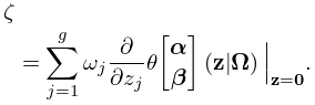
38: 31.9 Orthogonality

… ►

31.9.3 $${\theta }_m={(1-{\mathrm{e}}^{2\pi \mathrm{i}\gamma })(1-{\mathrm{e}}^{2\pi \mathrm{i}\delta }){\zeta }^{\gamma }{(1-\zeta )}^{\delta }{(\zeta -a)}^{ϵ}\frac{f_0(q,\zeta )}{f_1(q,\zeta )}\frac{\partial }{\partial q}𝒲\left\{f_0(q,\zeta ),f_1(q,\zeta )\right\}|}_{q=q_m},$$

ⓘ

Defines:

${\theta }_m$: normalization constant (locally)

Symbols:

$𝒲$: Wronskian, $\pi$: the ratio of the circumference of a circle to its diameter, $\mathrm{e}$: base of natural logarithm, $\mathrm{i}$: imaginary unit, $\frac{\partial f}{\partial x}$: partial derivative of $f$ with respect to $x$ , $\partial x$: partial differential of $x$ , $\gamma$: real or complex parameter, $\delta$: real or complex parameter, $ϵ$: real or complex parameter, $m$: nonnegative integer, $a$: complex parameter, $q$: real or complex parameter, $\zeta$: point and $f_0(q_m,z)$, $f_1(q_m,z)$: coefficients

Permalink:

http://dlmf.nist.gov/31.9.E3

Encodings:

pMML, png, TeX

See also:

Annotations for §31.9(i), §31.9 and Ch.31

…

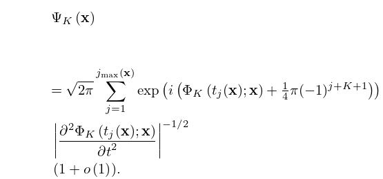
39: 36.11 Leading-Order Asymptotics

… ►

36.11.2 $${\mathrm{\Psi }}_K\left(𝐱\right)=\sqrt{2\pi }\sum _{j=1}^{j_{\max }(𝐱)}\exp \left(\mathrm{i}\left({\mathrm{\Phi }}_K(t_j(𝐱);𝐱)+\frac{1}{4}\pi {(-1)}^{j+K+1}\right)\right){\left|\frac{{\partial }^2{\mathrm{\Phi }}_K(t_j(𝐱);𝐱)}{{\partial t}^2}\right|}^{-1/2}(1+o\left(1\right)).$$

ⓘ

Symbols:

${\mathrm{\Psi }}_K\left(𝐱\right)$: canonical integral function, $\pi$: the ratio of the circumference of a circle to its diameter, ${\mathrm{\Phi }}_K(t;𝐱)$: cuspoid catastrophe of codimension $K$ , $\exp z$: exponential function, $\mathrm{i}$: imaginary unit, $o\left(x\right)$: order less than, $\frac{\partial f}{\partial x}$: partial derivative of $f$ with respect to $x$ , $\partial x$: partial differential of $x$ , $t$: variable, $K$: codimension and $t_j(𝐱)$: solutions

Permalink:

http://dlmf.nist.gov/36.11.E2

Encodings:

pMML, png, TeX

See also:

Annotations for §36.11 and Ch.36

…

40: 35.7 Gaussian Hypergeometric Function of Matrix Argument

… ►

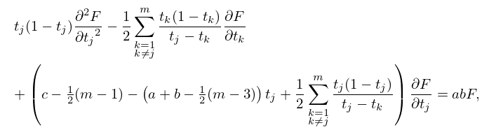
§35.7(iii) Partial Differential Equations

… ►Subject to the conditions (a)–(c), the function $f(𝐓)={}_2{}^{}F_1^{}(a,b;c;𝐓)$ is the unique solution of each partial differential equation ►

35.7.9 $$t_j(1-t_j)\frac{{\partial }^{2}F}{{\partial t_j}^2}-\frac{1}{2}\sum _{\begin{array}{c}k=1\\ k\ne j\end{array}}^m\frac{t_k(1-t_k)}{t_j-t_k}\frac{\partial F}{\partial t_k}+\left(c-\frac{1}{2}(m-1)-\left(a+b-\frac{1}{2}(m-3)\right)t_j+\frac{1}{2}\sum _{\begin{array}{c}k=1\\ k\ne j\end{array}}^m\frac{t_j(1-t_j)}{t_j-t_k}\right)\frac{\partial F}{\partial t_j}=abF,$$

ⓘ

Symbols:

$\frac{\partial f}{\partial x}$: partial derivative of $f$ with respect to $x$ , $\partial x$: partial differential of $x$ , $a$: complex variable, $t_j$: eigenvalues of $𝐓$ , $b$: complex variable, $c$: complex variable, $j$: nonnegative integer, $k$: nonnegative integer and $m$: positive integer

Referenced by:

§35.7(iii)

Permalink:

http://dlmf.nist.gov/35.7.E9

Encodings:

pMML, png, TeX

See also:

Annotations for §35.7(iii), §35.7 and Ch.35

… ►Systems of partial differential equations for the ${}_0{}^{}F_1^{}$ (defined in §35.8) and ${}_1{}^{}F_1^{}$ functions of matrix argument can be obtained by applying (35.8.9) and (35.8.10) to (35.7.9). …