of type 2

SearchAdvancedHelp

(0.006 seconds)

11—20 of 97 matching pages

11: Bibliography S

… ►

Bounds for ratios of modified Bessel functions and associated Turán-type inequalities. J. Math. Anal. Appl. 374 (2), pp. 516–528.

ⓘ

External Links:

ISSN 0022-247X, Document, FullText, MathReview (Beyza Caliskan Aslan), ZentralBlatt

Referenced by:

§10.37, §10.37.

Encodings:

BibTeX

… ►

On inequalities of the Turán type. Math. Scand. 2, pp. 65–73.

ⓘ

External Links:

ISSN 0025-5521, FullText, MathReview (G. Szegő), ZentralBlatt

Referenced by:

§18.14(ii).

Encodings:

BibTeX

…

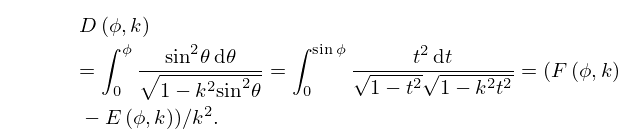
12: 19.2 Definitions

… ►

19.2.6 $$D(\varphi ,k)={\int }_0^{\varphi }\frac{{\sin }^2\theta d\theta }{\sqrt{1-k^2{\sin }^2\theta }}={\int }_0^{\sin \varphi }\frac{t^{2}dt}{\sqrt{1-t^2}\sqrt{1-k^2{t}^2}}=(F(\varphi ,k)-E(\varphi ,k))/k^2.$$

ⓘ

Defines:

$D(\varphi ,k)$: incomplete elliptic integral of Legendre’s type

Symbols:

$dx$: differential of $x$ , $F(\varphi ,k)$: Legendre’s incomplete elliptic integral of the first kind, $E(\varphi ,k)$: Legendre’s incomplete elliptic integral of the second kind, $\int$: integral, $\sin z$: sine function, $\varphi$: real or complex argument and $k$: real or complex modulus

Referenced by:

§19.25(i), §19.36(i)

Permalink:

http://dlmf.nist.gov/19.2.E6

Encodings:

pMML, png, TeX

See also:

Annotations for §19.2(ii), §19.2 and Ch.19

…

13: Bibliography P

… ►

A Kummer-type transformation for a ${}_2{}^{}F_2^{}$ hypergeometric function. J. Comput. Appl. Math. 173 (2), pp. 379–382.

ⓘ

External Links:

ISSN 0377-0427, Document, MathReview (P. Anandani), ZentralBlatt

Referenced by:

§16.6.

Encodings:

BibTeX

…

14: 8.10 Inequalities

… ►For further inequalities of these types see Qi and Mei (1999) and Neuman (2013). … ►For $n=1,2,\mathrm{\dots }$, … ►

$B_1={\displaystyle \frac{x+1}{x+2-a}},$

►

$A_2={\displaystyle \frac{x(x+3-a)}{x^2+2(2-a)x+(1-a)(2-a)}},$

►

$B_2={\displaystyle \frac{x^2+(5-a)x+2}{x^2+2(3-a)x+(2-a)(3-a)}}.$

…

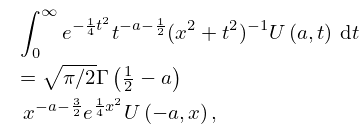
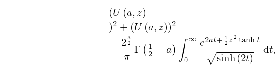
15: 12.12 Integrals

… ►

12.12.3 $${\int }_0^{\mathrm{\infty }}{\mathrm{e}}^{-\frac{1}{4}{t}^2}{t}^{-a-\frac{1}{2}}{(x^2+t^2)}^{-1}U(a,t)dt=\sqrt{\pi /2}\mathrm{\Gamma }\left(\frac{1}{2}-a\right)x^{-a-\frac{3}{2}}{\mathrm{e}}^{\frac{1}{4}{x}^2}U(-a,x),$$ .

ⓘ

Symbols:

$\mathrm{\Gamma }\left(z\right)$: gamma function, $\pi$: the ratio of the circumference of a circle to its diameter, $dx$: differential of $x$ , $\mathrm{e}$: base of natural logarithm, $\int$: integral, $U(a,z)$: parabolic cylinder function, $\mathrm{\Re }$: real part, $x$: real variable and $a$: real or complex parameter

Permalink:

http://dlmf.nist.gov/12.12.E3

Encodings:

pMML, png, TeX

See also:

Annotations for §12.12 and Ch.12

►

Nicholson-type Integral

►

12.12.4 $${(U(a,z))}^2+{(\overline{U}(a,z))}^2=\frac{2^{\frac{3}{2}}}{\pi }\mathrm{\Gamma }\left(\frac{1}{2}-a\right){\int }_0^{\mathrm{\infty }}\frac{{\mathrm{e}}^{2at+\frac{1}{2}{z}^2\tanh t}}{\sqrt{\sinh \left(2t\right)}}dt,$$ .

ⓘ

Symbols:

$\mathrm{\Gamma }\left(z\right)$: gamma function, $\pi$: the ratio of the circumference of a circle to its diameter, $dx$: differential of $x$ , $\mathrm{e}$: base of natural logarithm, $\sinh z$: hyperbolic sine function, $\tanh z$: hyperbolic tangent function, $\int$: integral, $U(a,z)$: parabolic cylinder function, $\overline{U}(a,x)$: parabolic cylinder function, $\mathrm{\Re }$: real part, $z$: complex variable and $a$: real or complex parameter

Notes:

See Durand (1975).

Referenced by:

§12.12

Permalink:

http://dlmf.nist.gov/12.12.E4

Encodings:

pMML, png, TeX

See also:

Annotations for §12.12, §12.12 and Ch.12

►When $z$ $(=x)$ is real the left-hand side equals ${(F(a,x))}^2$; compare (12.2.22). … ►For compendia of integrals see Erdélyi et al. (1953b, v. 2, pp. 121–122), Erdélyi et al. (1954a, b, v. 1, pp. 60–61, 115, 210–211, and 336; v. 2, pp. 76–80, 115, 151, 171, and 395–398), Gradshteyn and Ryzhik (2000, §7.7), Magnus et al. (1966, pp. 330–331), Marichev (1983, pp. 190–191), Oberhettinger (1974, pp. 144–145), Oberhettinger (1990, pp. 106–108 and 192), Oberhettinger and Badii (1973, pp. 181–185), Prudnikov et al. (1986b, pp. 36–37, 155–168, 243–246, 289–290, 327–328, 419–420, and 619), Prudnikov et al. (1992a, §3.11), and Prudnikov et al. (1992b, §3.11). …

16: 10.32 Integral Representations

… ►

10.32.2 $$I_{\nu }\left(z\right)=\frac{{(\frac{1}{2}z)}^{\nu }}{{\pi }^{\frac{1}{2}}\mathrm{\Gamma }\left(\nu +\frac{1}{2}\right)}{\int }_0^{\pi }{\mathrm{e}}^{\pm z\cos \theta }{(\sin \theta )}^{2\nu }d\theta =\frac{{(\frac{1}{2}z)}^{\nu }}{{\pi }^{\frac{1}{2}}\mathrm{\Gamma }\left(\nu +\frac{1}{2}\right)}{\int }_{-1}^1{(1-t^2)}^{\nu -\frac{1}{2}}{\mathrm{e}}^{\pm zt}dt,$$ $\mathrm{\Re }\nu >-\frac{1}{2}$.

ⓘ

Symbols:

$\mathrm{\Gamma }\left(z\right)$: gamma function, $\pi$: the ratio of the circumference of a circle to its diameter, $\cos z$: cosine function, $dx$: differential of $x$ , $\mathrm{e}$: base of natural logarithm, $\int$: integral, $I_{\nu }\left(z\right)$: modified Bessel function of the first kind, $\mathrm{\Re }$: real part, $\sin z$: sine function, $z$: complex variable and $\nu$: complex parameter

A&S Ref:

9.6.18

Permalink:

http://dlmf.nist.gov/10.32.E2

Encodings:

pMML, png, TeX

See also:

Annotations for §10.32(i), §10.32 and Ch.10

… ►

10.32.8 $$K_{\nu }\left(z\right)=\frac{{\pi }^{\frac{1}{2}}{(\frac{1}{2}z)}^{\nu }}{\mathrm{\Gamma }\left(\nu +\frac{1}{2}\right)}{\int }_0^{\mathrm{\infty }}{\mathrm{e}}^{-z\cosh t}{(\sinh t)}^{2\nu }dt=\frac{{\pi }^{\frac{1}{2}}{(\frac{1}{2}z)}^{\nu }}{\mathrm{\Gamma }\left(\nu +\frac{1}{2}\right)}{\int }_1^{\mathrm{\infty }}{\mathrm{e}}^{-zt}{(t^2-1)}^{\nu -\frac{1}{2}}dt,$$ $\mathrm{\Re }\nu >-\frac{1}{2}$, .

ⓘ

Symbols:

$\mathrm{\Gamma }\left(z\right)$: gamma function, $\pi$: the ratio of the circumference of a circle to its diameter, $dx$: differential of $x$ , $\mathrm{e}$: base of natural logarithm, $\cosh z$: hyperbolic cosine function, $\sinh z$: hyperbolic sine function, $\int$: integral, $K_{\nu }\left(z\right)$: modified Bessel function of the second kind, $\mathrm{ph}$: phase, $\mathrm{\Re }$: real part, $z$: complex variable and $\nu$: complex parameter

A&S Ref:

9.6.23

Referenced by:

§10.74(iii)

Permalink:

http://dlmf.nist.gov/10.32.E8

Encodings:

pMML, png, TeX

See also:

Annotations for §10.32(i), §10.32 and Ch.10

… ►

Mellin–Barnes Type

… ►In (10.32.14) the integration contour separates the poles of $\mathrm{\Gamma }\left(t\right)$ from the poles of $\mathrm{\Gamma }\left(\frac{1}{2}-t-\nu \right)\mathrm{\Gamma }\left(\frac{1}{2}-t+\nu \right)$. … ►

Mellin–Barnes Type

…

17: Bibliography T

… ►

Numerical algorithms for uniform Airy-type asymptotic expansions. Numer. Algorithms 15 (2), pp. 207–225.

ⓘ

External Links:

ISSN 1017-1398, Document, MathReview, ZentralBlatt

Referenced by:

§10.19(iii), §10.20(i), §10.74(i).

Encodings:

BibTeX

…

18: 7.7 Integral Representations

… ►Integrals of the type $\int {\mathrm{e}}^{-z^2}R(z)dz$, where $R(z)$ is an arbitrary rational function, can be written in closed form in terms of the error functions and elementary functions. …

19: 13.16 Integral Representations

… ►In this subsection see §§10.2(ii), 10.25(ii) for the functions $J_{2\mu }$, $I_{2\mu }$, and $K_{2\mu }$, and §§15.1, 15.2(i) for ${}_2{}^{}𝐅_1^{}$. … ►

§13.16(iii) Mellin–Barnes Integrals

►If $\frac{1}{2}+\mu -\kappa \ne 0,-1,-2,\mathrm{\dots }$, then … ►If $\frac{1}{2}\pm \mu -\kappa \ne 0,-1,-2,\mathrm{\dots }$, then …where the contour of integration passes all the poles of $\mathrm{\Gamma }\left(\frac{1}{2}+\mu +t\right)\mathrm{\Gamma }\left(\frac{1}{2}-\mu +t\right)$ on the right-hand side.

20: 10.9 Integral Representations

… ►Also, ${(t^2-1)}^{\nu -\frac{1}{2}}$ is continuous on the path, and takes its principal value at the intersection with the interval $(1,\mathrm{\infty })$. … ►

Mellin–Barnes Type Integrals

… ►where the integration path passes to the left of $t=0,1,2,\mathrm{\dots }$. … ►For (10.9.22)–(10.9.25) and further integrals of this type see Paris and Kaminski (2001, pp. 114–116). … ►

Mellin–Barnes Type

…