of the third kind

SearchAdvancedHelp

(0.006 seconds)

21—30 of 95 matching pages

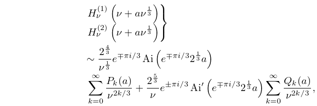
21: 10.19 Asymptotic Expansions for Large Order

… ►

10.19.2 $$Y_{\nu }\left(z\right)\sim -\mathrm{i}{H}_{\nu }^{(1)}\left(z\right)\sim \mathrm{i}{H}_{\nu }^{(2)}\left(z\right)\sim -\sqrt{\frac{2}{\pi \nu }}{\left(\frac{\mathrm{e}z}{2\nu }\right)}^{-\nu }.$$

ⓘ

Symbols:

$Y_{\nu }\left(z\right)$: Bessel function of the second kind, $H_{\nu }^{(1)}\left(z\right)$: Bessel function of the third kind (or Hankel function), $H_{\nu }^{(2)}\left(z\right)$: Bessel function of the third kind (or Hankel function), $\sim$: asymptotic equality, $\pi$: the ratio of the circumference of a circle to its diameter, $\mathrm{e}$: base of natural logarithm, $\mathrm{i}$: imaginary unit, $z$: complex variable and $\nu$: complex parameter

A&S Ref:

9.3.1

Referenced by:

§10.41(i)

Permalink:

http://dlmf.nist.gov/10.19.E2

Encodings:

pMML, png, TeX

See also:

Annotations for §10.19(i), §10.19 and Ch.10

… ►

10.19.9 $$\begin{array}{c}{H}_{\nu }^{(1)}\left(\nu +a{\nu }^{\frac{1}{3}}\right)\\ H_{\nu }^{(2)}\left(\nu +a{\nu }^{\frac{1}{3}}\right)\end{array}\}\sim \frac{2^{\frac{4}{3}}}{{\nu }^{\frac{1}{3}}}{\mathrm{e}}^{\mp \pi \mathrm{i}/3}\mathrm{Ai}\left({\mathrm{e}}^{\mp \pi \mathrm{i}/3}{2}^{\frac{1}{3}}a\right)\sum _{k=0}^{\mathrm{\infty }}\frac{P_k(a)}{{\nu }^{2k/3}}+\frac{2^{\frac{5}{3}}}{\nu }{\mathrm{e}}^{\pm \pi \mathrm{i}/3}{\mathrm{Ai}}^{\prime }\left({\mathrm{e}}^{\mp \pi \mathrm{i}/3}{2}^{\frac{1}{3}}a\right)\sum _{k=0}^{\mathrm{\infty }}\frac{Q_k(a)}{{\nu }^{2k/3}},$$

ⓘ

Symbols:

$\mathrm{Ai}\left(z\right)$: Airy function, $H_{\nu }^{(1)}\left(z\right)$: Bessel function of the third kind (or Hankel function), $H_{\nu }^{(2)}\left(z\right)$: Bessel function of the third kind (or Hankel function), $\sim$: Poincaré asymptotic expansion, $\pi$: the ratio of the circumference of a circle to its diameter, $\mathrm{e}$: base of natural logarithm, $\mathrm{i}$: imaginary unit, $k$: nonnegative integer, $\nu$: complex parameter, $P_k(a)$: polynomial coefficient and $Q_k(a)$: polynomial coefficient

Permalink:

http://dlmf.nist.gov/10.19.E9

Encodings:

pMML, png, TeX

Correction (effective with 1.0.27):

Originally the polynomials $P_k(a)$, $Q_k(a)$ were incorrectly described as Legendre polynomials and integer-degree, zero-order associated Legendre functions of the second kind respectively.

See also:

Annotations for §10.19(iii), §10.19 and Ch.10

… ►

10.19.13 $$\begin{array}{c}H_{\nu }^{(1)}{}_{}{}^{\prime }\left(\nu +a{\nu }^{\frac{1}{3}}\right)\\ H_{\nu }^{(2)}{}_{}{}^{\prime }\left(\nu +a{\nu }^{\frac{1}{3}}\right)\end{array}\}\sim -\frac{2^{\frac{5}{3}}}{{\nu }^{\frac{2}{3}}}{\mathrm{e}}^{\pm \pi \mathrm{i}/3}{\mathrm{Ai}}^{\prime }\left({\mathrm{e}}^{\mp \pi \mathrm{i}/3}{2}^{\frac{1}{3}}a\right)\sum _{k=0}^{\mathrm{\infty }}\frac{R_k(a)}{{\nu }^{2k/3}}+\frac{2^{\frac{4}{3}}}{{\nu }^{\frac{4}{3}}}{\mathrm{e}}^{\mp \pi \mathrm{i}/3}\mathrm{Ai}\left({\mathrm{e}}^{\mp \pi \mathrm{i}/3}{2}^{\frac{1}{3}}a\right)\sum _{k=0}^{\mathrm{\infty }}\frac{S_k(a)}{{\nu }^{2k/3}},$$

ⓘ

Symbols:

$\mathrm{Ai}\left(z\right)$: Airy function, $H_{\nu }^{(1)}\left(z\right)$: Bessel function of the third kind (or Hankel function), $H_{\nu }^{(2)}\left(z\right)$: Bessel function of the third kind (or Hankel function), $\sim$: Poincaré asymptotic expansion, $\pi$: the ratio of the circumference of a circle to its diameter, $\mathrm{e}$: base of natural logarithm, $\mathrm{i}$: imaginary unit, $k$: nonnegative integer, $\nu$: complex parameter, $R_k(a)$: polynomial coefficient and $S_k(a)$: polynomial coefficient

Permalink:

http://dlmf.nist.gov/10.19.E13

Encodings:

pMML, png, TeX

See also:

Annotations for §10.19(iii), §10.19 and Ch.10

…

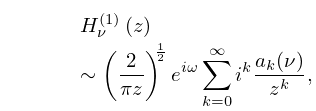
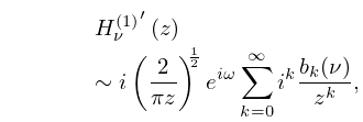
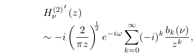
22: 10.17 Asymptotic Expansions for Large Argument

… ►

10.17.5 $$H_{\nu }^{(1)}\left(z\right)\sim {\left(\frac{2}{\pi z}\right)}^{\frac{1}{2}}{\mathrm{e}}^{\mathrm{i}\omega }\sum _{k=0}^{\mathrm{\infty }}{\mathrm{i}}^k\frac{a_k(\nu )}{z^k},$$ $-\pi +\delta \le \mathrm{ph}z\le 2\pi -\delta$,

ⓘ

Symbols:

$H_{\nu }^{(1)}\left(z\right)$: Bessel function of the third kind (or Hankel function), $\sim$: Poincaré asymptotic expansion, $\pi$: the ratio of the circumference of a circle to its diameter, $\mathrm{e}$: base of natural logarithm, $\mathrm{i}$: imaginary unit, $\mathrm{ph}$: phase, $k$: nonnegative integer, $z$: complex variable, $\nu$: complex parameter, $\delta$: small positive constant, $a_k(\nu )$: polynomial coefficient and $\omega$

A&S Ref:

9.2.7

Referenced by:

§10.17(i), §10.17(iii), §10.17(iv), §10.41(v)

Permalink:

http://dlmf.nist.gov/10.17.E5

Encodings:

pMML, png, TeX

See also:

Annotations for §10.17(i), §10.17 and Ch.10

►

10.17.6 $$H_{\nu }^{(2)}\left(z\right)\sim {\left(\frac{2}{\pi z}\right)}^{\frac{1}{2}}{\mathrm{e}}^{-\mathrm{i}\omega }\sum _{k=0}^{\mathrm{\infty }}{(-\mathrm{i})}^k\frac{a_k(\nu )}{z^k},$$ $-2\pi +\delta \le \mathrm{ph}z\le \pi -\delta$,

ⓘ

Symbols:

$H_{\nu }^{(2)}\left(z\right)$: Bessel function of the third kind (or Hankel function), $\sim$: Poincaré asymptotic expansion, $\pi$: the ratio of the circumference of a circle to its diameter, $\mathrm{e}$: base of natural logarithm, $\mathrm{i}$: imaginary unit, $\mathrm{ph}$: phase, $k$: nonnegative integer, $z$: complex variable, $\nu$: complex parameter, $\delta$: small positive constant, $a_k(\nu )$: polynomial coefficient and $\omega$

A&S Ref:

9.2.8

Referenced by:

§10.17(i), §10.17(iii), §10.17(iv), §10.41(v), §10.49(i), §10.61(v)

Permalink:

http://dlmf.nist.gov/10.17.E6

Encodings:

pMML, png, TeX

See also:

Annotations for §10.17(i), §10.17 and Ch.10

… ►

10.17.11 $$H_{\nu }^{(1)}{}_{}{}^{\prime }\left(z\right)\sim \mathrm{i}{\left(\frac{2}{\pi z}\right)}^{\frac{1}{2}}{\mathrm{e}}^{\mathrm{i}\omega }\sum _{k=0}^{\mathrm{\infty }}{\mathrm{i}}^k\frac{b_k(\nu )}{z^k},$$ $-\pi +\delta \le \mathrm{ph}z\le 2\pi -\delta$,

ⓘ

Symbols:

$H_{\nu }^{(1)}\left(z\right)$: Bessel function of the third kind (or Hankel function), $\sim$: Poincaré asymptotic expansion, $\pi$: the ratio of the circumference of a circle to its diameter, $\mathrm{e}$: base of natural logarithm, $\mathrm{i}$: imaginary unit, $\mathrm{ph}$: phase, $k$: nonnegative integer, $z$: complex variable, $\nu$: complex parameter, $\delta$: small positive constant, $\omega$ and $b_k(\nu )$: polynomial coefficient

A&S Ref:

9.2.13

Referenced by:

§10.18(iii)

Permalink:

http://dlmf.nist.gov/10.17.E11

Encodings:

pMML, png, TeX

See also:

Annotations for §10.17(ii), §10.17 and Ch.10

►

10.17.12 $$H_{\nu }^{(2)}{}_{}{}^{\prime }\left(z\right)\sim -\mathrm{i}{\left(\frac{2}{\pi z}\right)}^{\frac{1}{2}}{\mathrm{e}}^{-\mathrm{i}\omega }\sum _{k=0}^{\mathrm{\infty }}{(-\mathrm{i})}^k\frac{b_k(\nu )}{z^k},$$ $-2\pi +\delta \le \mathrm{ph}z\le \pi -\delta$.

ⓘ

Symbols:

$H_{\nu }^{(2)}\left(z\right)$: Bessel function of the third kind (or Hankel function), $\sim$: Poincaré asymptotic expansion, $\pi$: the ratio of the circumference of a circle to its diameter, $\mathrm{e}$: base of natural logarithm, $\mathrm{i}$: imaginary unit, $\mathrm{ph}$: phase, $k$: nonnegative integer, $z$: complex variable, $\nu$: complex parameter, $\delta$: small positive constant, $\omega$ and $b_k(\nu )$: polynomial coefficient

A&S Ref:

9.2.14

Referenced by:

§10.18(iii)

Permalink:

http://dlmf.nist.gov/10.17.E12

Encodings:

pMML, png, TeX

See also:

Annotations for §10.17(ii), §10.17 and Ch.10

… ►

10.17.13 $$\begin{array}{c}{H}_{\nu }^{(1)}\left(z\right)\\ H_{\nu }^{(2)}\left(z\right)\end{array}\}={\left(\frac{2}{\pi z}\right)}^{\frac{1}{2}}{\mathrm{e}}^{\pm \mathrm{i}\omega }\left(\sum _{k=0}^{\mathrm{\ell }-1}{(\pm \mathrm{i})}^k\frac{a_k(\nu )}{z^k}+R_{\mathrm{\ell }}^{\pm }(\nu ,z)\right),$$ $\mathrm{\ell }=1,2,\mathrm{\dots }$.

ⓘ

Symbols:

$H_{\nu }^{(1)}\left(z\right)$: Bessel function of the third kind (or Hankel function), $H_{\nu }^{(2)}\left(z\right)$: Bessel function of the third kind (or Hankel function), $\pi$: the ratio of the circumference of a circle to its diameter, $\mathrm{e}$: base of natural logarithm, $\mathrm{i}$: imaginary unit, $k$: nonnegative integer, $z$: complex variable, $\nu$: complex parameter, $a_k(\nu )$: polynomial coefficient, $\omega$ and $R_{\mathrm{\ell }}^{\pm }(\nu ,z)$: remainder

Referenced by:

§10.17(iv), §10.17(v)

Permalink:

http://dlmf.nist.gov/10.17.E13

Encodings:

pMML, png, TeX

See also:

Annotations for §10.17(iv), §10.17 and Ch.10

…

23: 11.2 Definitions

… ►

11.2.13 $$w={𝐇}_{\nu }\left(z\right)+A{J}_{\nu }\left(z\right)+B{H}_{\nu }^{(1)}\left(z\right),$$

ⓘ

Symbols:

$J_{\nu }\left(z\right)$: Bessel function of the first kind, $H_{\nu }^{(1)}\left(z\right)$: Bessel function of the third kind (or Hankel function), ${𝐇}_{\nu }\left(z\right)$: Struve function, $z$: complex variable, $\nu$: real or complex order, $A$: arbitrary constant and $B$: arbitrary constant

Referenced by:

§11.2(iii)

Permalink:

http://dlmf.nist.gov/11.2.E13

Encodings:

pMML, png, TeX

See also:

Annotations for §11.2(iii), §11.2 and Ch.11

►

11.2.14 $$w={𝐇}_{\nu }\left(z\right)+A{J}_{\nu }\left(z\right)+B{H}_{\nu }^{(2)}\left(z\right),$$

ⓘ

Symbols:

$J_{\nu }\left(z\right)$: Bessel function of the first kind, $H_{\nu }^{(2)}\left(z\right)$: Bessel function of the third kind (or Hankel function), ${𝐇}_{\nu }\left(z\right)$: Struve function, $z$: complex variable, $\nu$: real or complex order, $A$: arbitrary constant and $B$: arbitrary constant

Referenced by:

§11.2(iii)

Permalink:

http://dlmf.nist.gov/11.2.E14

Encodings:

pMML, png, TeX

See also:

Annotations for §11.2(iii), §11.2 and Ch.11

►

11.2.15 $$w={𝐊}_{\nu }\left(z\right)+A{H}_{\nu }^{(1)}\left(z\right)+B{H}_{\nu }^{(2)}\left(z\right).$$

ⓘ

Symbols:

$H_{\nu }^{(1)}\left(z\right)$: Bessel function of the third kind (or Hankel function), $H_{\nu }^{(2)}\left(z\right)$: Bessel function of the third kind (or Hankel function), ${𝐊}_{\nu }\left(z\right)$: Struve function, $z$: complex variable, $\nu$: real or complex order, $A$: arbitrary constant and $B$: arbitrary constant

Referenced by:

§11.2(iii), §11.2(iii)

Permalink:

http://dlmf.nist.gov/11.2.E15

Encodings:

pMML, png, TeX

See also:

Annotations for §11.2(iii), §11.2 and Ch.11

…

24: 19.7 Connection Formulas

… ►

$\mathrm{\Pi }(\varphi ,{\alpha }^2,k_1)=k\mathrm{\Pi }(\beta ,k^2{\alpha }^2,k),$ $k_1=1/k$, $\sin \beta =k_1\sin \varphi \le 1$.

… ►

$$\mathrm{\Pi }(\mathrm{i}\varphi ,{\alpha }^2,k)=\mathrm{i}\left(F(\psi ,k^{\prime })-{\alpha }^2\mathrm{\Pi }(\psi ,1-{\alpha }^2,k^{\prime })\right)/(1-{\alpha }^2).$$

… ►

§19.7(iii) Change of Parameter of $\mathrm{\Pi }(\varphi ,{\alpha }^2,k)$

►There are three relations connecting $\mathrm{\Pi }(\varphi ,{\alpha }^2,k)$ and $\mathrm{\Pi }(\varphi ,{\omega }^2,k)$, where ${\omega }^2$ is a rational function of ${\alpha }^2$. … ►The first of the three relations maps each circular region onto itself and each hyperbolic region onto the other; in particular, it gives the Cauchy principal value of $\mathrm{\Pi }(\varphi ,{\alpha }^2,k)$ when ${\alpha }^2>{\csc }^2\varphi$ (see (19.6.5) for the complete case). …

25: 10.73 Physical Applications

… ►The functions ${𝗃}_n\left(x\right)$, ${𝗒}_n\left(x\right)$, ${𝗁}_n^{(1)}\left(x\right)$, and ${𝗁}_n^{(2)}\left(x\right)$ arise in the solution (again by separation of variables) of the Helmholtz equation in spherical coordinates $\rho ,\theta ,\varphi$ (§1.5(ii)): …With the spherical harmonic $Y_{\mathrm{\ell },m}\left(\theta ,\varphi \right)$ defined as in §14.30(i), the solutions are of the form $f=g_{\mathrm{\ell }}(k\rho )Y_{\mathrm{\ell },m}\left(\theta ,\varphi \right)$ with $g_{\mathrm{\ell }}={𝗃}_{\mathrm{\ell }}$, ${𝗒}_{\mathrm{\ell }}$, ${𝗁}_{\mathrm{\ell }}^{(1)}$, or ${𝗁}_{\mathrm{\ell }}^{(2)}$, depending on the boundary conditions. …

26: 10.42 Zeros

… ►Properties of the zeros of $I_{\nu }\left(z\right)$ and $K_{\nu }\left(z\right)$ may be deduced from those of $J_{\nu }\left(z\right)$ and $H_{\nu }^{(1)}\left(z\right)$, respectively, by application of the transformations (10.27.6) and (10.27.8). …

27: 10.6 Recurrence Relations and Derivatives

… ►

$H_0^{(1)}{}_{}{}^{\prime }\left(z\right)=-H_1^{(1)}\left(z\right),$ $H_0^{(2)}{}_{}{}^{\prime }\left(z\right)=-H_1^{(2)}\left(z\right).$

…

28: 10.51 Recurrence Relations and Derivatives

… ►Let $f_n(z)$ denote any of ${𝗃}_n\left(z\right)$, ${𝗒}_n\left(z\right)$, ${𝗁}_n^{(1)}\left(z\right)$, or ${𝗁}_n^{(2)}\left(z\right)$. …

29: 10.9 Integral Representations

… ►

10.9.10 $$H_{\nu }^{(1)}\left(z\right)=\frac{{\mathrm{e}}^{-\frac{1}{2}\nu \pi \mathrm{i}}}{\pi \mathrm{i}}{\int }_{-\mathrm{\infty }}^{\mathrm{\infty }}{\mathrm{e}}^{\mathrm{i}z\cosh t-\nu t}dt,$$ ,

ⓘ

Symbols:

$H_{\nu }^{(1)}\left(z\right)$: Bessel function of the third kind (or Hankel function), $\pi$: the ratio of the circumference of a circle to its diameter, $dx$: differential of $x$ , $\mathrm{e}$: base of natural logarithm, $\cosh z$: hyperbolic cosine function, $\mathrm{i}$: imaginary unit, $\int$: integral, $\mathrm{ph}$: phase, $z$: complex variable and $\nu$: complex parameter

Referenced by:

§10.9(i)

Permalink:

http://dlmf.nist.gov/10.9.E10

Encodings:

pMML, png, TeX

See also:

Annotations for §10.9(i), §10.9(i), §10.9 and Ch.10

►

10.9.11 $$H_{\nu }^{(2)}\left(z\right)=-\frac{{\mathrm{e}}^{\frac{1}{2}\nu \pi \mathrm{i}}}{\pi \mathrm{i}}{\int }_{-\mathrm{\infty }}^{\mathrm{\infty }}{\mathrm{e}}^{-\mathrm{i}z\cosh t-\nu t}dt,$$ .

ⓘ

Symbols:

$H_{\nu }^{(2)}\left(z\right)$: Bessel function of the third kind (or Hankel function), $\pi$: the ratio of the circumference of a circle to its diameter, $dx$: differential of $x$ , $\mathrm{e}$: base of natural logarithm, $\cosh z$: hyperbolic cosine function, $\mathrm{i}$: imaginary unit, $\int$: integral, $\mathrm{ph}$: phase, $z$: complex variable and $\nu$: complex parameter

Referenced by:

§10.9(i)

Permalink:

http://dlmf.nist.gov/10.9.E11

Encodings:

pMML, png, TeX

See also:

Annotations for §10.9(i), §10.9(i), §10.9 and Ch.10

… ►

10.9.15 $${\left(\frac{z+\zeta }{z-\zeta }\right)}^{\frac{1}{2}\nu }{H}_{\nu }^{(1)}\left({(z^2-{\zeta }^2)}^{\frac{1}{2}}\right)=\frac{1}{\pi \mathrm{i}}{\mathrm{e}}^{-\frac{1}{2}\nu \pi \mathrm{i}}{\int }_{-\mathrm{\infty }}^{\mathrm{\infty }}{\mathrm{e}}^{\mathrm{i}z\cosh t+\mathrm{i}\zeta \sinh t-\nu t}dt,$$ $\mathrm{\Im }\left(z\pm \zeta \right)>0$,

ⓘ

Symbols:

$H_{\nu }^{(1)}\left(z\right)$: Bessel function of the third kind (or Hankel function), $\pi$: the ratio of the circumference of a circle to its diameter, $dx$: differential of $x$ , $\mathrm{e}$: base of natural logarithm, $\cosh z$: hyperbolic cosine function, $\sinh z$: hyperbolic sine function, $\mathrm{\Im }$: imaginary part, $\mathrm{i}$: imaginary unit, $\int$: integral, $z$: complex variable and $\nu$: complex parameter

Referenced by:

§10.9(i)

Permalink:

http://dlmf.nist.gov/10.9.E15

Encodings:

pMML, png, TeX

See also:

Annotations for §10.9(i), §10.9(i), §10.9 and Ch.10

… ►

$H_{\nu }^{(1)}\left(z\right)={\displaystyle \frac{1}{\pi \mathrm{i}}}{\displaystyle {\int }_{-\mathrm{\infty }}^{\mathrm{\infty }+\pi \mathrm{i}}}{\mathrm{e}}^{z\sinh t-\nu t}dt,$

►

$H_{\nu }^{(2)}\left(z\right)=-{\displaystyle \frac{1}{\pi \mathrm{i}}}{\displaystyle {\int }_{-\mathrm{\infty }}^{\mathrm{\infty }-\pi \mathrm{i}}}{\mathrm{e}}^{z\sinh t-\nu t}dt.$

…

30: 10.74 Methods of Computation

… ►For $z\in ℂ$ the function $H_{\nu }^{(1)}\left(z\right)$, for example, can always be computed in a stable manner in the sector $0\le \mathrm{ph}z\le \pi$ by integrating along rays towards the origin. … ►For evaluation of the Hankel functions $H_{\nu }^{(1)}\left(z\right)$ and $H_{\nu }^{(2)}\left(z\right)$ for complex values of $\nu$ and $z$ based on the integral representations (10.9.18) see Remenets (1973). …