odd%20part
(0.002 seconds)
21—30 of 400 matching pages
21: 30.9 Asymptotic Approximations and Expansions
22: 10.59 Integrals
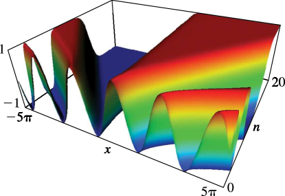
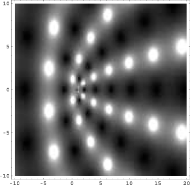
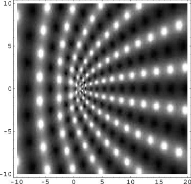
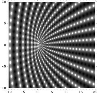
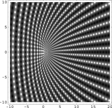
23: 22.3 Graphics
 ►
►
 ►
►
 ►
►
 ►
►
24: 9.18 Tables
Zhang and Jin (1996, p. 337) tabulates , , , for to 8S and for to 9D.
Woodward and Woodward (1946) tabulates the real and imaginary parts of , , , for , . Precision is 4D.
Sherry (1959) tabulates , , , , ; 20S.
Corless et al. (1992) gives the real and imaginary parts of for ; 14S.
25: 20.10 Integrals
26: 10.75 Tables
Achenbach (1986) tabulates , , , , , 20D or 18–20S.
Zhang and Jin (1996, pp. 185–195) tabulates , , , , , , 5, 10, 25, 50, 100, 9S; , , , , , , , 8S; real and imaginary parts of , , , , , , , , 8S.
Bickley et al. (1952) tabulates or , or , , (.01 or .1) 10(.1) 20, 8S; , , , or , 10S.
Zhang and Jin (1996, pp. 240–250) tabulates , , , , , , 9S; , , , , , 10, 30, 50, 100, , , , , , , 5, 10, 50, 8S; real and imaginary parts of , , , , , 20(10)50, 100, , , 8S.
Zhang and Jin (1996, pp. 296–305) tabulates , , , , , , , , , 50, 100, , 5, 10, 25, 50, 100, 8S; , , , (Riccati–Bessel functions and their derivatives), , 50, 100, , 5, 10, 25, 50, 100, 8S; real and imaginary parts of , , , , , , , , , 20(10)50, 100, , , 8S. (For the notation replace by , , , , respectively.)


