normalized

SearchAdvancedHelp

(0.001 seconds)

21—30 of 108 matching pages

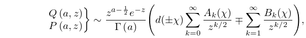
21: 8.12 Uniform Asymptotic Expansions for Large Parameter

… ►

8.12.3 $$P(a,z)=\frac{1}{2}\mathrm{erfc}\left(-\eta \sqrt{a/2}\right)-S(a,\eta ),$$

ⓘ

Symbols:

$\mathrm{erfc}z$: complementary error function, $P(a,z)$: normalized incomplete gamma function, $z$: complex variable, $a$: parameter, $\eta (\lambda )$ and $S(a,\eta )$: function

Permalink:

http://dlmf.nist.gov/8.12.E3

Encodings:

pMML, png, TeX

See also:

Annotations for §8.12 and Ch.8

►

8.12.4 $$Q(a,z)=\frac{1}{2}\mathrm{erfc}\left(\eta \sqrt{a/2}\right)+S(a,\eta ),$$

ⓘ

Symbols:

$\mathrm{erfc}z$: complementary error function, $Q(a,z)$: normalized incomplete gamma function, $z$: complex variable, $a$: parameter, $\eta (\lambda )$ and $S(a,\eta )$: function

Referenced by:

§8.12

Permalink:

http://dlmf.nist.gov/8.12.E4

Encodings:

pMML, png, TeX

See also:

Annotations for §8.12 and Ch.8

… ►

8.12.15 $$Q(a,a)\sim \frac{1}{2}+\frac{1}{\sqrt{2\pi a}}\sum _{k=0}^{\mathrm{\infty }}{c}_k(0)a^{-k},$$ $|\mathrm{ph}a|\le \pi -\delta$,

ⓘ

Symbols:

$\sim$: Poincaré asymptotic expansion, $\pi$: the ratio of the circumference of a circle to its diameter, $Q(a,z)$: normalized incomplete gamma function, $\mathrm{ph}$: phase, $a$: parameter, $k$: nonnegative integer, $\delta$: small positive constant and $c_k(\eta )$: coefficients

Permalink:

http://dlmf.nist.gov/8.12.E15

Encodings:

pMML, png, TeX

See also:

Annotations for §8.12 and Ch.8

… ►

8.12.18 $$\begin{array}{c}Q(a,z)\\ P(a,z)\end{array}\}\sim \frac{z^{a-\frac{1}{2}}{\mathrm{e}}^{-z}}{\mathrm{\Gamma }\left(a\right)}\left(d(\pm \chi )\sum _{k=0}^{\mathrm{\infty }}\frac{A_k(\chi )}{z^{k/2}}\mp \sum _{k=1}^{\mathrm{\infty }}\frac{B_k(\chi )}{z^{k/2}}\right),$$

ⓘ

Symbols:

$\mathrm{\Gamma }\left(z\right)$: gamma function, $\sim$: Poincaré asymptotic expansion, $\mathrm{e}$: base of natural logarithm, $P(a,z)$: normalized incomplete gamma function, $Q(a,z)$: normalized incomplete gamma function, $z$: complex variable, $a$: parameter, $k$: nonnegative integer, $\chi$ , $d(\pm \chi )$ , $A_k(\chi )$ and $B_k(\chi )$

Referenced by:

§8.12, Erratum (V1.0.16) for Equation (8.12.18)

Permalink:

http://dlmf.nist.gov/8.12.E18

Encodings:

pMML, png, TeX

Errata (effective with 1.0.16):

The original $\pm$ in front of the second summation was replaced by $\mp$ to correct an error in Paris (2002b); for details see https://arxiv.org/abs/1611.00548.

Reported 2017-01-28 by Richard Paris

See also:

Annotations for §8.12 and Ch.8

… ►

8.12.21 $$Q(a,x)=q$$

ⓘ

Symbols:

$Q(a,z)$: normalized incomplete gamma function and $a$: parameter

Permalink:

http://dlmf.nist.gov/8.12.E21

Encodings:

pMML, png, TeX

See also:

Annotations for §8.12, §8.12 and Ch.8

…

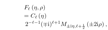
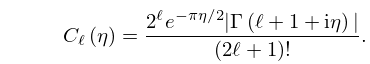
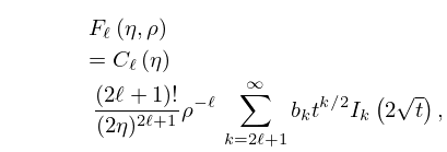
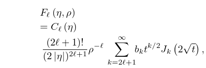
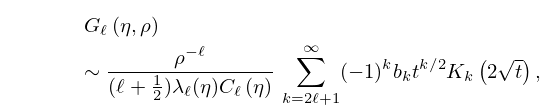
22: 33.2 Definitions and Basic Properties

… ►

33.2.3 $$F_{\mathrm{\ell }}(\eta ,\rho )=C_{\mathrm{\ell }}\left(\eta \right)2^{-\mathrm{\ell }-1}{(\mp \mathrm{i})}^{\mathrm{\ell }+1}{M}_{\pm \mathrm{i}\eta ,\mathrm{\ell }+\frac{1}{2}}\left(\pm 2\mathrm{i}\rho \right),$$

ⓘ

Defines:

$F_{\mathrm{\ell }}(\eta ,\rho )$: regular Coulomb radial function

Symbols:

$C_{\mathrm{\ell }}\left(\eta \right)$: normalizing constant for Coulomb radial functions, $M_{\kappa ,\mu }\left(z\right)$: Whittaker confluent hypergeometric function, $\mathrm{i}$: imaginary unit, $\mathrm{\ell }$: nonnegative integer, $\rho$: nonnegative real variable and $\eta$: real parameter

Referenced by:

§13.18(vi), §33.2(ii)

Permalink:

http://dlmf.nist.gov/33.2.E3

Encodings:

pMML, png, TeX

See also:

Annotations for §33.2(ii), §33.2 and Ch.33

… ►

33.2.5 $$C_{\mathrm{\ell }}\left(\eta \right)=\frac{2^{\mathrm{\ell }}{\mathrm{e}}^{-\pi \eta /2}|\mathrm{\Gamma }\left(\mathrm{\ell }+1+\mathrm{i}\eta \right)|}{(2\mathrm{\ell }+1)!}.$$

ⓘ

Defines:

$C_{\mathrm{\ell }}\left(\eta \right)$: normalizing constant for Coulomb radial functions

Symbols:

$\mathrm{\Gamma }\left(z\right)$: gamma function, $\pi$: the ratio of the circumference of a circle to its diameter, $\mathrm{e}$: base of natural logarithm, $!$: factorial (as in $n!$), $\mathrm{i}$: imaginary unit, $\mathrm{\ell }$: nonnegative integer and $\eta$: real parameter

A&S Ref:

14.1.7

Referenced by:

§33.10(ii), §33.10(iii), §33.16(i)

Permalink:

http://dlmf.nist.gov/33.2.E5

Encodings:

pMML, png, TeX

See also:

Annotations for §33.2(ii), §33.2 and Ch.33

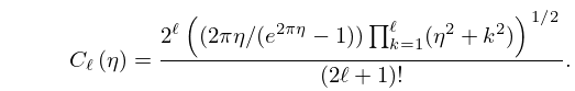
… ► $F_{\mathrm{\ell }}(\eta ,\rho )$ is a real and analytic function of $\rho$ on the open interval , and also an analytic function of $\eta$ when . ►The normalizing constant $C_{\mathrm{\ell }}\left(\eta \right)$ is always positive, and has the alternative form ►

33.2.6 $$C_{\mathrm{\ell }}\left(\eta \right)=\frac{2^{\mathrm{\ell }}{\left((2\pi \eta /({\mathrm{e}}^{2\pi \eta }-1)){\prod }_{k=1}^{\mathrm{\ell }}({\eta }^2+k^2)\right)}^{1/2}}{(2\mathrm{\ell }+1)!}.$$

ⓘ

Symbols:

$C_{\mathrm{\ell }}\left(\eta \right)$: normalizing constant for Coulomb radial functions, $\pi$: the ratio of the circumference of a circle to its diameter, $\mathrm{e}$: base of natural logarithm, $!$: factorial (as in $n!$), $k$: nonnegative integer, $\mathrm{\ell }$: nonnegative integer and $\eta$: real parameter

Referenced by:

§33.13, §33.16(i)

Permalink:

http://dlmf.nist.gov/33.2.E6

Encodings:

pMML, png, TeX

See also:

Annotations for §33.2(ii), §33.2 and Ch.33

…

23: 1.18 Linear Second Order Differential Operators and Eigenfunction Expansions

… ►These are based on the Liouville normal form of (1.13.29). … ► … ►Applying equations (1.18.29) and (1.18.30), the complete set of normalized eigenfunctions being … ► … ►Then orthogonality and normalization relations are …

24: 3.6 Linear Difference Equations

… ►It therefore remains to apply a normalizing factor $\mathrm{\Lambda }$. The process is then repeated with a higher value of $N$, and the normalized solutions compared. … ►The normalizing factor $\mathrm{\Lambda }$ can be the true value of $w_0$ divided by its trial value, or $\mathrm{\Lambda }$ can be chosen to satisfy a known property of the wanted solution of the form … … ►For further information, including a more general form of normalizing condition, other examples, convergence proofs, and error analyses, see Olver (1967a), Olver and Sookne (1972), and Wimp (1984, Chapter 6). …

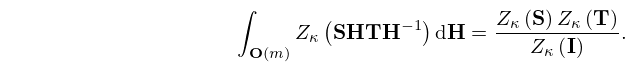
25: 35.4 Partitions and Zonal Polynomials

… ►

35.4.3 $$Z_{\kappa }\left(𝐓\right)=Z_{\kappa }\left(𝐈\right){\left|𝐓\right|}^{k_m}\underset{𝐎(m)}{\int }\prod _{j=1}^{m-1}{|{(𝐇𝐓{𝐇}^{-1})}_j|}^{k_j-k_{j+1}}\mathrm{d}𝐇,$$ $𝐓\in 𝓢$.

ⓘ

Symbols:

$\in$: element of, $\int$: integral, $Z_{\kappa }\left(𝐓\right)$: zonal polynomial, $𝐈$: $m\times m$ identity matrix, $𝓢$: space of real symmetric $m\times m$ matrices, $𝐓$: real symmetric $m\times m$ matrix, $\left|𝐗\right|$: determinant of $𝐗$ , $|{(𝐗)}_j|$: $j$th principal minor of $𝐗$ , $𝐎(m)$: space of $m\times m$ orthogonal matrices, $𝐇$: orthogonal $m\times m$ matrix, $\mathrm{d}𝐇$: normalized Haar measure on $𝐎(m)$ , $j$: nonnegative integer, $k$: nonnegative integer, $m$: positive integer and $\kappa$: vector of nonnegative integers

Referenced by:

§35.4(i)

Permalink:

http://dlmf.nist.gov/35.4.E3

Encodings:

pMML, png, TeX

See also:

Annotations for §35.4(i), §35.4 and Ch.35

… ►

Normalization

… ►

35.4.7 $${\int }_{𝐎(m)}{Z}_{\kappa }\left(𝐒𝐇𝐓{𝐇}^{-1}\right)\mathrm{d}𝐇=\frac{Z_{\kappa }\left(𝐒\right)Z_{\kappa }\left(𝐓\right)}{Z_{\kappa }\left(𝐈\right)}.$$

ⓘ

Symbols:

$\int$: integral, $Z_{\kappa }\left(𝐓\right)$: zonal polynomial, $𝐈$: $m\times m$ identity matrix, $𝐒$: real symmetric $m\times m$ matrix, $𝐓$: real symmetric $m\times m$ matrix, $𝐎(m)$: space of $m\times m$ orthogonal matrices, $𝐇$: orthogonal $m\times m$ matrix, $\mathrm{d}𝐇$: normalized Haar measure on $𝐎(m)$ , $m$: positive integer and $\kappa$: vector of nonnegative integers

Referenced by:

§35.9

Permalink:

http://dlmf.nist.gov/35.4.E7

Encodings:

pMML, png, TeX

See also:

Annotations for §35.4(ii), §35.4(ii), §35.4 and Ch.35

…

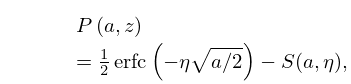
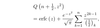
26: 8.4 Special Values

… ►

8.4.9 $$P(n+1,z)=1-{\mathrm{e}}^{-z}{e}_n(z),$$

ⓘ

Symbols:

$\mathrm{e}$: base of natural logarithm, $P(a,z)$: normalized incomplete gamma function, $z$: complex variable, $n$: nonnegative integer and $e_n(z)$: functions

A&S Ref:

6.5.13

Permalink:

http://dlmf.nist.gov/8.4.E9

Encodings:

pMML, png, TeX

See also:

Annotations for §8.4 and Ch.8

►

8.4.10 $$Q(n+1,z)={\mathrm{e}}^{-z}{e}_n(z),$$

ⓘ

Symbols:

$\mathrm{e}$: base of natural logarithm, $Q(a,z)$: normalized incomplete gamma function, $z$: complex variable, $n$: nonnegative integer and $e_n(z)$: functions

Permalink:

http://dlmf.nist.gov/8.4.E10

Encodings:

pMML, png, TeX

See also:

Annotations for §8.4 and Ch.8

… ►

8.4.14 $$Q(n+\frac{1}{2},z^2)=\mathrm{erfc}\left(z\right)+\frac{{\mathrm{e}}^{-z^2}}{\sqrt{\pi }}\sum _{k=1}^n\frac{z^{2k-1}}{{\left(\frac{1}{2}\right)}_k},$$

ⓘ

Symbols:

${\left(a\right)}_n$: Pochhammer’s symbol (or shifted factorial), $\pi$: the ratio of the circumference of a circle to its diameter, $\mathrm{erfc}z$: complementary error function, $\mathrm{e}$: base of natural logarithm, $Q(a,z)$: normalized incomplete gamma function, $z$: complex variable, $k$: nonnegative integer and $n$: nonnegative integer

Referenced by:

§8.4

Permalink:

http://dlmf.nist.gov/8.4.E14

Encodings:

pMML, png, TeX

See also:

Annotations for §8.4 and Ch.8

…

27: 22.18 Mathematical Applications

… ►The special case $y^2=(1-x^2)(1-k^2{x}^2)$ is in Jacobian normal form. For any two points $(x_1,y_1)$ and $(x_2,y_2)$ on this curve, their sum $(x_3,y_3)$, always a third point on the curve, is defined by the Jacobi–Abel addition law …

28: 30.16 Methods of Computation

… ►If ${\lambda }_n^m\left({\gamma }^2\right)$ is known, then we can compute ${\mathrm{𝖯𝗌}}_n^m(x,{\gamma }^2)$ (not normalized) by solving the differential equation (30.2.1) numerically with initial conditions $w(0)=1$, $w^{\prime }(0)=0$ if $n-m$ is even, or $w(0)=0$, $w^{\prime }(0)=1$ if $n-m$ is odd. … ►The coefficients $a_{n,r}^m({\gamma }^2)$ are computed as the recessive solution of (30.8.4) (§3.6), and normalized via (30.8.5). … ►Form the eigenvector ${[e_{1,d},e_{2,d},\mathrm{\dots },e_{d,d}]}^{\mathrm{T}}$ of $𝐀$ associated with the eigenvalue ${\alpha }_{p,d}$, $p=\lfloor \frac{1}{2}(n-m)\rfloor +1$, normalized according to …

29: 33.9 Expansions in Series of Bessel Functions

… ►

33.9.3 $$F_{\mathrm{\ell }}(\eta ,\rho )=C_{\mathrm{\ell }}\left(\eta \right)\frac{(2\mathrm{\ell }+1)!}{{(2\eta )}^{2\mathrm{\ell }+1}}{\rho }^{-\mathrm{\ell }}\sum _{k=2\mathrm{\ell }+1}^{\mathrm{\infty }}{b}_k{t}^{k/2}{I}_k\left(2\sqrt{t}\right),$$ $\eta >0$,

ⓘ

Symbols:

$C_{\mathrm{\ell }}\left(\eta \right)$: normalizing constant for Coulomb radial functions, $!$: factorial (as in $n!$), $I_{\nu }\left(z\right)$: modified Bessel function of the first kind, $F_{\mathrm{\ell }}(\eta ,\rho )$: regular Coulomb radial function, $k$: nonnegative integer, $\mathrm{\ell }$: nonnegative integer, $\rho$: nonnegative real variable, $\eta$: real parameter, $t$: parameter and $b_k$: coefficient

A&S Ref:

14.4.1

Referenced by:

§33.9(ii), §33.9(ii)

Permalink:

http://dlmf.nist.gov/33.9.E3

Encodings:

pMML, png, TeX

See also:

Annotations for §33.9(ii), §33.9 and Ch.33

►

33.9.4 $$F_{\mathrm{\ell }}(\eta ,\rho )=C_{\mathrm{\ell }}\left(\eta \right)\frac{(2\mathrm{\ell }+1)!}{{(2\left|\eta \right|)}^{2\mathrm{\ell }+1}}{\rho }^{-\mathrm{\ell }}\sum _{k=2\mathrm{\ell }+1}^{\mathrm{\infty }}{b}_k{t}^{k/2}{J}_k\left(2\sqrt{t}\right),$$ .

ⓘ

Symbols:

$J_{\nu }\left(z\right)$: Bessel function of the first kind, $C_{\mathrm{\ell }}\left(\eta \right)$: normalizing constant for Coulomb radial functions, $!$: factorial (as in $n!$), $F_{\mathrm{\ell }}(\eta ,\rho )$: regular Coulomb radial function, $k$: nonnegative integer, $\mathrm{\ell }$: nonnegative integer, $\rho$: nonnegative real variable, $\eta$: real parameter, $t$: parameter and $b_k$: coefficient

Referenced by:

§33.9(ii), §33.9(ii)

Permalink:

http://dlmf.nist.gov/33.9.E4

Encodings:

pMML, png, TeX

See also:

Annotations for §33.9(ii), §33.9 and Ch.33

… ►

33.9.6 $$G_{\mathrm{\ell }}(\eta ,\rho )\sim \frac{{\rho }^{-\mathrm{\ell }}}{(\mathrm{\ell }+\frac{1}{2}){\lambda }_{\mathrm{\ell }}(\eta )C_{\mathrm{\ell }}\left(\eta \right)}\sum _{k=2\mathrm{\ell }+1}^{\mathrm{\infty }}{(-1)}^k{b}_k{t}^{k/2}{K}_k\left(2\sqrt{t}\right),$$

ⓘ

Symbols:

$C_{\mathrm{\ell }}\left(\eta \right)$: normalizing constant for Coulomb radial functions, $\sim$: asymptotic equality, $G_{\mathrm{\ell }}(\eta ,\rho )$: irregular Coulomb radial function, $K_{\nu }\left(z\right)$: modified Bessel function of the second kind, $k$: nonnegative integer, $\mathrm{\ell }$: nonnegative integer, $\rho$: nonnegative real variable, $\eta$: real parameter, $t$: parameter, $b_k$: coefficient and ${\lambda }_{\mathrm{\ell }}(\eta )$: coefficient

A&S Ref:

14.4.2

Referenced by:

§33.9(ii)

Permalink:

http://dlmf.nist.gov/33.9.E6

Encodings:

pMML, png, TeX

See also:

Annotations for §33.9(ii), §33.9 and Ch.33

…

30: 35.1 Special Notation

… ► ►►►

$a,b$	complex variables.
…
$\mathrm{d}𝐇$	normalized Haar measure on $𝐎(m)$.
…

…