normal%20values

SearchAdvancedHelp

(0.000 seconds)

21—30 of 467 matching pages

21: 29.21 Tables

… ►

Arscott and Khabaza (1962) tabulates the coefficients of the polynomials $P$ in Table 29.12.1 (normalized so that the numerically largest coefficient is unity, i.e. monic polynomials), and the corresponding eigenvalues $h$ for $k^2=0.1(.1)0.9$, $n=1(1)30$. Equations from §29.6 can be used to transform to the normalization adopted in this chapter. Precision is 6S.

22: 14.33 Tables

… ►

Zhang and Jin (1996, Chapter 4) tabulates ${𝖯}_n\left(x\right)$ for $n=2(1)5,10$, $x=0(.1)1$, 7D; ${𝖯}_n\left(\cos \theta \right)$ for $n=1(1)4,10$, $\theta =0(5^{\circ }){90}^{\circ }$, 8D; ${𝖰}_n\left(x\right)$ for $n=0(1)2,10$, $x=0(.1)0.9$, 8S; ${𝖰}_n\left(\cos \theta \right)$ for $n=0(1)3,10$, $\theta =0(5^{\circ }){90}^{\circ }$, 8D; ${𝖯}_n^m\left(x\right)$ for $m=1(1)4$, $n-m=0(1)2$, $n=10$, $x=0,0.5$, 8S; ${𝖰}_n^m\left(x\right)$ for $m=1(1)4$, $n=0(1)2,10$, 8S; ${𝖯}_{\nu }^m\left(\cos \theta \right)$ for $m=0(1)3$, $\nu =0(.25)5$, $\theta =0({15}^{\circ }){90}^{\circ }$, 5D; $P_n\left(x\right)$ for $n=2(1)5,10$, $x=1(1)10$, 7S; $Q_n\left(x\right)$ for $n=0(1)2,10$, $x=2(1)10$, 8S. Corresponding values of the derivative of each function are also included, as are 6D values of the first 5 $\nu$-zeros of ${𝖯}_{\nu }^m\left(\cos \theta \right)$ and of its derivative for $m=0(1)4$, $\theta ={10}^{\circ },{30}^{\circ },{150}^{\circ }$.

►

Belousov (1962) tabulates ${𝖯}_n^m\left(\cos \theta \right)$ (normalized) for $m=0(1)36$, $n-m=0(1)56$, $\theta =0({2.5}^{\circ }){90}^{\circ }$, 6D.

►

Žurina and Karmazina (1964, 1965) tabulate the conical functions ${𝖯}_{-\frac{1}{2}+\mathrm{i}\tau }\left(x\right)$ for $\tau =0(.01)50$, $x=-0.9(.1)0.9$, 7S; $P_{-\frac{1}{2}+\mathrm{i}\tau }\left(x\right)$ for $\tau =0(.01)50$, $x=1.1(.1)2(.2)5(.5)10(10)60$, 7D. Auxiliary tables are included to facilitate computation for larger values of $\tau$ when .

►

Žurina and Karmazina (1963) tabulates the conical functions ${𝖯}_{-\frac{1}{2}+\mathrm{i}\tau }^1\left(x\right)$ for $\tau =0(.01)25$, $x=-0.9(.1)0.9$, 7S; $P_{-\frac{1}{2}+\mathrm{i}\tau }^1\left(x\right)$ for $\tau =0(.01)25$, $x=1.1(.1)2(.2)5(.5)10(10)60$, 7S. Auxiliary tables are included to assist computation for larger values of $\tau$ when .

…

23: 18.39 Applications in the Physical Sciences

… ►Brief mention of non-unit normalized solutions in the case of mixed spectra appear, but as these solutions are not OP’s details appear elsewhere, as referenced. … ►By Table 18.3.1#12 the normalized stationary states and corresponding eigenvalues are … ►There is no need for a normalization constant here, as appropriate constants already appear in §18.36(vi). … ►Explicit normalization is given for the second, third, and fourth of these, paragraphs c) and d), below. … ►thus recapitulating, for $Z=1$, line 11 of Table 18.8.1, now shown with explicit normalization for the measure $dr$. …

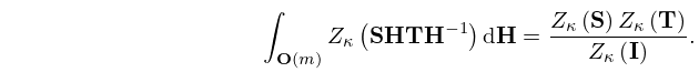
24: 35.4 Partitions and Zonal Polynomials

… ►

35.4.3 $$Z_{\kappa }\left(𝐓\right)=Z_{\kappa }\left(𝐈\right){\left|𝐓\right|}^{k_m}\underset{𝐎(m)}{\int }\prod _{j=1}^{m-1}{|{(𝐇𝐓{𝐇}^{-1})}_j|}^{k_j-k_{j+1}}\mathrm{d}𝐇,$$ $𝐓\in 𝓢$.

ⓘ

Symbols:

$\in$: element of, $\int$: integral, $Z_{\kappa }\left(𝐓\right)$: zonal polynomial, $𝐈$: $m\times m$ identity matrix, $𝓢$: space of real symmetric $m\times m$ matrices, $𝐓$: real symmetric $m\times m$ matrix, $\left|𝐗\right|$: determinant of $𝐗$ , $|{(𝐗)}_j|$: $j$th principal minor of $𝐗$ , $𝐎(m)$: space of $m\times m$ orthogonal matrices, $𝐇$: orthogonal $m\times m$ matrix, $\mathrm{d}𝐇$: normalized Haar measure on $𝐎(m)$ , $j$: nonnegative integer, $k$: nonnegative integer, $m$: positive integer and $\kappa$: vector of nonnegative integers

Referenced by:

§35.4(i)

Permalink:

http://dlmf.nist.gov/35.4.E3

Encodings:

pMML, png, TeX

See also:

Annotations for §35.4(i), §35.4 and Ch.35

… ►

Normalization

… ►

Mean-Value

►

35.4.7 $${\int }_{𝐎(m)}{Z}_{\kappa }\left(𝐒𝐇𝐓{𝐇}^{-1}\right)\mathrm{d}𝐇=\frac{Z_{\kappa }\left(𝐒\right)Z_{\kappa }\left(𝐓\right)}{Z_{\kappa }\left(𝐈\right)}.$$

ⓘ

Symbols:

$\int$: integral, $Z_{\kappa }\left(𝐓\right)$: zonal polynomial, $𝐈$: $m\times m$ identity matrix, $𝐒$: real symmetric $m\times m$ matrix, $𝐓$: real symmetric $m\times m$ matrix, $𝐎(m)$: space of $m\times m$ orthogonal matrices, $𝐇$: orthogonal $m\times m$ matrix, $\mathrm{d}𝐇$: normalized Haar measure on $𝐎(m)$ , $m$: positive integer and $\kappa$: vector of nonnegative integers

Referenced by:

§35.9

Permalink:

http://dlmf.nist.gov/35.4.E7

Encodings:

pMML, png, TeX

See also:

Annotations for §35.4(ii), §35.4(ii), §35.4 and Ch.35

…

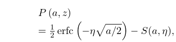
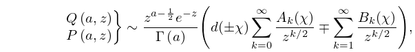
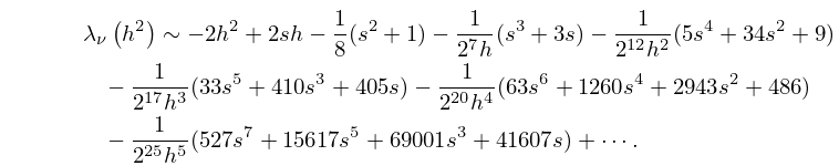
25: 8.12 Uniform Asymptotic Expansions for Large Parameter

… ►

8.12.3 $$P(a,z)=\frac{1}{2}\mathrm{erfc}\left(-\eta \sqrt{a/2}\right)-S(a,\eta ),$$

ⓘ

Symbols:

$\mathrm{erfc}z$: complementary error function, $P(a,z)$: normalized incomplete gamma function, $z$: complex variable, $a$: parameter, $\eta (\lambda )$ and $S(a,\eta )$: function

Permalink:

http://dlmf.nist.gov/8.12.E3

Encodings:

pMML, png, TeX

See also:

Annotations for §8.12 and Ch.8

►

8.12.4 $$Q(a,z)=\frac{1}{2}\mathrm{erfc}\left(\eta \sqrt{a/2}\right)+S(a,\eta ),$$

ⓘ

Symbols:

$\mathrm{erfc}z$: complementary error function, $Q(a,z)$: normalized incomplete gamma function, $z$: complex variable, $a$: parameter, $\eta (\lambda )$ and $S(a,\eta )$: function

Referenced by:

§8.12

Permalink:

http://dlmf.nist.gov/8.12.E4

Encodings:

pMML, png, TeX

See also:

Annotations for §8.12 and Ch.8

… ►For numerical values of $d_{k,n}$ to 30D for $k=0(1)9$ and $n=0(1)N_k$, where $N_k=28-4\lfloor k/2\rfloor$, see DiDonato and Morris (1986). … ►

8.12.18 $$\begin{array}{c}Q(a,z)\\ P(a,z)\end{array}\}\sim \frac{z^{a-\frac{1}{2}}{\mathrm{e}}^{-z}}{\mathrm{\Gamma }\left(a\right)}\left(d(\pm \chi )\sum _{k=0}^{\mathrm{\infty }}\frac{A_k(\chi )}{z^{k/2}}\mp \sum _{k=1}^{\mathrm{\infty }}\frac{B_k(\chi )}{z^{k/2}}\right),$$

ⓘ

Symbols:

$\mathrm{\Gamma }\left(z\right)$: gamma function, $\sim$: Poincaré asymptotic expansion, $\mathrm{e}$: base of natural logarithm, $P(a,z)$: normalized incomplete gamma function, $Q(a,z)$: normalized incomplete gamma function, $z$: complex variable, $a$: parameter, $k$: nonnegative integer, $\chi$ , $d(\pm \chi )$ , $A_k(\chi )$ and $B_k(\chi )$

Referenced by:

§8.12, Erratum (V1.0.16) for Equation (8.12.18)

Permalink:

http://dlmf.nist.gov/8.12.E18

Encodings:

pMML, png, TeX

Errata (effective with 1.0.16):

The original $\pm$ in front of the second summation was replaced by $\mp$ to correct an error in Paris (2002b); for details see https://arxiv.org/abs/1611.00548.

Reported 2017-01-28 by Richard Paris

See also:

Annotations for §8.12 and Ch.8

… ►

8.12.21 $$Q(a,x)=q$$

ⓘ

Symbols:

$Q(a,z)$: normalized incomplete gamma function and $a$: parameter

Permalink:

http://dlmf.nist.gov/8.12.E21

Encodings:

pMML, png, TeX

See also:

Annotations for §8.12, §8.12 and Ch.8

…

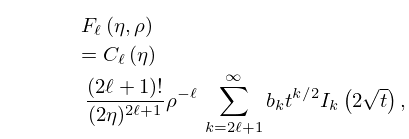
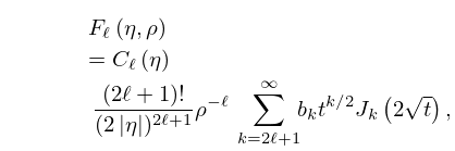
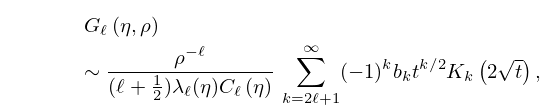
26: 33.9 Expansions in Series of Bessel Functions

… ►The series (33.9.1) converges for all finite values of $\eta$ and $\rho$. … ►

33.9.3 $$F_{\mathrm{\ell }}(\eta ,\rho )=C_{\mathrm{\ell }}\left(\eta \right)\frac{(2\mathrm{\ell }+1)!}{{(2\eta )}^{2\mathrm{\ell }+1}}{\rho }^{-\mathrm{\ell }}\sum _{k=2\mathrm{\ell }+1}^{\mathrm{\infty }}{b}_k{t}^{k/2}{I}_k\left(2\sqrt{t}\right),$$ $\eta >0$,

ⓘ

Symbols:

$C_{\mathrm{\ell }}\left(\eta \right)$: normalizing constant for Coulomb radial functions, $!$: factorial (as in $n!$), $I_{\nu }\left(z\right)$: modified Bessel function of the first kind, $F_{\mathrm{\ell }}(\eta ,\rho )$: regular Coulomb radial function, $k$: nonnegative integer, $\mathrm{\ell }$: nonnegative integer, $\rho$: nonnegative real variable, $\eta$: real parameter, $t$: parameter and $b_k$: coefficient

A&S Ref:

14.4.1

Referenced by:

§33.9(ii), §33.9(ii)

Permalink:

http://dlmf.nist.gov/33.9.E3

Encodings:

pMML, png, TeX

See also:

Annotations for §33.9(ii), §33.9 and Ch.33

►

33.9.4 $$F_{\mathrm{\ell }}(\eta ,\rho )=C_{\mathrm{\ell }}\left(\eta \right)\frac{(2\mathrm{\ell }+1)!}{{(2\left|\eta \right|)}^{2\mathrm{\ell }+1}}{\rho }^{-\mathrm{\ell }}\sum _{k=2\mathrm{\ell }+1}^{\mathrm{\infty }}{b}_k{t}^{k/2}{J}_k\left(2\sqrt{t}\right),$$ .

ⓘ

Symbols:

$J_{\nu }\left(z\right)$: Bessel function of the first kind, $C_{\mathrm{\ell }}\left(\eta \right)$: normalizing constant for Coulomb radial functions, $!$: factorial (as in $n!$), $F_{\mathrm{\ell }}(\eta ,\rho )$: regular Coulomb radial function, $k$: nonnegative integer, $\mathrm{\ell }$: nonnegative integer, $\rho$: nonnegative real variable, $\eta$: real parameter, $t$: parameter and $b_k$: coefficient

Referenced by:

§33.9(ii), §33.9(ii)

Permalink:

http://dlmf.nist.gov/33.9.E4

Encodings:

pMML, png, TeX

See also:

Annotations for §33.9(ii), §33.9 and Ch.33

… ►The series (33.9.3) and (33.9.4) converge for all finite positive values of $\left|\eta \right|$ and $\rho$. … ►

33.9.6 $$G_{\mathrm{\ell }}(\eta ,\rho )\sim \frac{{\rho }^{-\mathrm{\ell }}}{(\mathrm{\ell }+\frac{1}{2}){\lambda }_{\mathrm{\ell }}(\eta )C_{\mathrm{\ell }}\left(\eta \right)}\sum _{k=2\mathrm{\ell }+1}^{\mathrm{\infty }}{(-1)}^k{b}_k{t}^{k/2}{K}_k\left(2\sqrt{t}\right),$$

ⓘ

Symbols:

$C_{\mathrm{\ell }}\left(\eta \right)$: normalizing constant for Coulomb radial functions, $\sim$: asymptotic equality, $G_{\mathrm{\ell }}(\eta ,\rho )$: irregular Coulomb radial function, $K_{\nu }\left(z\right)$: modified Bessel function of the second kind, $k$: nonnegative integer, $\mathrm{\ell }$: nonnegative integer, $\rho$: nonnegative real variable, $\eta$: real parameter, $t$: parameter, $b_k$: coefficient and ${\lambda }_{\mathrm{\ell }}(\eta )$: coefficient

A&S Ref:

14.4.2

Referenced by:

§33.9(ii)

Permalink:

http://dlmf.nist.gov/33.9.E6

Encodings:

pMML, png, TeX

See also:

Annotations for §33.9(ii), §33.9 and Ch.33

…

27: Bibliography M

… ►

Rational approximations, software and test methods for sine and cosine integrals. Numer. Algorithms 12 (3-4), pp. 259–272.

ⓘ

Notes:

Includes Fortran code, maximum accuracy 20S.

External Links:

ISSN 1017-1398, Document, MathReview, ZentralBlatt

Referenced by:

§6.13, 4th item, §6.21(ii).

Encodings:

BibTeX

… ►

Exact misclassification probabilities for plug-in normal quadratic discriminant functions. I. The equal-means case. J. Multivariate Anal. 77 (1), pp. 21–53.

ⓘ

External Links:

ISSN 0047-259X, Document, MathReview (Peter A. Lachenbruch), ZentralBlatt

Referenced by:

§35.9.

Encodings:

BibTeX

►

Exact misclassification probabilities for plug-in normal quadratic discriminant functions. II. The heterogeneous case. J. Multivariate Anal. 82 (2), pp. 299–330.

ⓘ

External Links:

ISSN 0047-259X, Document, MathReview (Peter A. Lachenbruch), ZentralBlatt

Referenced by:

§35.9.

Encodings:

BibTeX

… ►

Table of the ratio: Area to bounding ordinate, for any portion of normal curve. Biometrika 18, pp. 395–400.

ⓘ

External Links:

FullText, ZentralBlatt

Referenced by:

§7.8.

Encodings:

BibTeX

… ►

The $q$-analogue of the Laguerre polynomials. J. Math. Anal. Appl. 81 (1), pp. 20–47.

ⓘ

External Links:

ISSN 0022-247X, Document, MathReview (R. A. Askey), ZentralBlatt

Referenced by:

§18.27(v).

Encodings:

BibTeX

…

28: 8.3 Graphics

… ►In the graphics shown in this subsection, height corresponds to the absolute value of the function and color to the phase. … ►

►

►

Figure 8.3.8: $\mathrm{\Gamma }(0.25,x+\mathrm{i}y)$, $-3\le x\le 3$, $-3\le y\le 3$. Principal value. … Magnify 3D Help

►

►

►

Figure 8.3.9: $\gamma (0.25,x+\mathrm{i}y)$, $-3\le x\le 3$, $-3\le y\le 3$. Principal value. … Magnify 3D Help

… ►

►

►

Figure 8.3.14: $\mathrm{\Gamma }(2.5,x+\mathrm{i}y)$, $-2.2\le x\le 3$, $-3\le y\le 3$. Principal value. … Magnify 3D Help

►

►

►

Figure 8.3.15: $\gamma (2.5,x+\mathrm{i}y)$, $-2.2\le x\le 3$, $-3\le y\le 3$. Principal value. … Magnify 3D Help

…

29: 24.20 Tables

… ►Abramowitz and Stegun (1964, Chapter 23) includes exact values of ${\sum }_{k=1}^m{k}^n$, $m=1(1)100$, $n=1(1)10$; ${\sum }_{k=1}^{\mathrm{\infty }}{k}^{-n}$, ${\sum }_{k=1}^{\mathrm{\infty }}{(-1)}^{k-1}{k}^{-n}$, ${\sum }_{k=0}^{\mathrm{\infty }}{(2k+1)}^{-n}$, $n=1,2,\mathrm{\dots }$, 20D; ${\sum }_{k=0}^{\mathrm{\infty }}{(-1)}^k{(2k+1)}^{-n}$, $n=1,2,\mathrm{\dots }$, 18D. ►Wagstaff (1978) gives complete prime factorizations of $N_n$ and $E_n$ for $n=20(2)60$ and $n=8(2)42$, respectively. …

30: 28.16 Asymptotic Expansions for Large $q$

§28.16 Asymptotic Expansions for Large $q$

… ►

28.16.1 $${\lambda }_{\nu }\left(h^2\right)\sim -2h^2+2sh-\frac{1}{8}(s^2+1)-\frac{1}{2^{7}h}(s^3+3s)-\frac{1}{2^{12}{h}^2}(5s^4+34s^2+9)-\frac{1}{2^{17}{h}^3}(33s^5+410s^3+405s)-\frac{1}{2^{20}{h}^4}(63s^6+1260s^4+2943s^2+486)-\frac{1}{2^{25}{h}^5}(527s^7+15617s^5+69001s^3+41607s)+\mathrm{\cdots }.$$

ⓘ

Symbols:

${\lambda }_{\nu +2n}\left(q\right)$: eigenvalues of Mathieu equation, $\sim$: Poincaré asymptotic expansion, $h$: parameter and $\nu$: complex parameter

Permalink:

http://dlmf.nist.gov/28.16.E1

Encodings:

pMML, png, TeX

See also:

Annotations for §28.16 and Ch.28

…