modulus

SearchAdvancedHelp

(0.001 seconds)

31—40 of 532 matching pages

31: 9.2 Differential Equation

… ►

9.2.10 $$\mathrm{Bi}\left(z\right)={\mathrm{e}}^{-\pi \mathrm{i}/6}\mathrm{Ai}\left(z{\mathrm{e}}^{-2\pi \mathrm{i}/3}\right)+{\mathrm{e}}^{\pi \mathrm{i}/6}\mathrm{Ai}\left(z{\mathrm{e}}^{2\pi \mathrm{i}/3}\right).$$

ⓘ

Symbols:

$\mathrm{Ai}\left(z\right)$: Airy function, $\mathrm{Bi}\left(z\right)$: Airy function, $\pi$: the ratio of the circumference of a circle to its diameter, $\mathrm{e}$: base of natural logarithm, $\mathrm{i}$: imaginary unit and $z$: complex variable

Proof sketch:

Derivable from Olver (1997b, p. 414).

A&S Ref:

10.4.6

Referenced by:

(9.10.19), (9.5.5)

Permalink:

http://dlmf.nist.gov/9.2.E10

Encodings:

pMML, png, TeX

See also:

Annotations for §9.2(v), §9.2 and Ch.9

… ►

9.2.12 $$\mathrm{Ai}\left(z\right)+{\mathrm{e}}^{-2\pi \mathrm{i}/3}\mathrm{Ai}\left(z{\mathrm{e}}^{-2\pi \mathrm{i}/3}\right)+{\mathrm{e}}^{2\pi \mathrm{i}/3}\mathrm{Ai}\left(z{\mathrm{e}}^{2\pi \mathrm{i}/3}\right)=0,$$

ⓘ

Symbols:

$\mathrm{Ai}\left(z\right)$: Airy function, $\pi$: the ratio of the circumference of a circle to its diameter, $\mathrm{e}$: base of natural logarithm, $\mathrm{i}$: imaginary unit and $z$: complex variable

Source:

Olver (1997b, (8.03), p. 414)

A&S Ref:

10.4.7

Permalink:

http://dlmf.nist.gov/9.2.E12

Encodings:

pMML, png, TeX

See also:

Annotations for §9.2(v), §9.2 and Ch.9

►

9.2.13 $$\mathrm{Bi}\left(z\right)+{\mathrm{e}}^{-2\pi \mathrm{i}/3}\mathrm{Bi}\left(z{\mathrm{e}}^{-2\pi \mathrm{i}/3}\right)+{\mathrm{e}}^{2\pi \mathrm{i}/3}\mathrm{Bi}\left(z{\mathrm{e}}^{2\pi \mathrm{i}/3}\right)=0.$$

ⓘ

Symbols:

$\mathrm{Bi}\left(z\right)$: Airy function, $\pi$: the ratio of the circumference of a circle to its diameter, $\mathrm{e}$: base of natural logarithm, $\mathrm{i}$: imaginary unit and $z$: complex variable

Proof sketch:

Derivable from Olver (1997b, p. 414).

A&S Ref:

10.4.8

Permalink:

http://dlmf.nist.gov/9.2.E13

Encodings:

pMML, png, TeX

See also:

Annotations for §9.2(v), §9.2 and Ch.9

►

9.2.14 $$\mathrm{Ai}\left(-z\right)={\mathrm{e}}^{\pi \mathrm{i}/3}\mathrm{Ai}\left(z{\mathrm{e}}^{\pi \mathrm{i}/3}\right)+{\mathrm{e}}^{-\pi \mathrm{i}/3}\mathrm{Ai}\left(z{\mathrm{e}}^{-\pi \mathrm{i}/3}\right),$$

ⓘ

Symbols:

$\mathrm{Ai}\left(z\right)$: Airy function, $\pi$: the ratio of the circumference of a circle to its diameter, $\mathrm{e}$: base of natural logarithm, $\mathrm{i}$: imaginary unit and $z$: complex variable

Source:

Olver (1997b, p. 414)

Permalink:

http://dlmf.nist.gov/9.2.E14

Encodings:

pMML, png, TeX

See also:

Annotations for §9.2(v), §9.2 and Ch.9

… ► $W=(1/w)dw/dz$, where $w$ is any nontrivial solution of (9.2.1). …

32: 19.13 Integrals of Elliptic Integrals

… ►

§19.13(i) Integration with Respect to the Modulus

…

33: 20.15 Tables

… ►This reference gives ${\theta }_j(x,q)$, $j=1,2,3,4$, and their logarithmic $x$-derivatives to 4D for $x/\pi =0(.1)1$, $\alpha =0(9^{\circ }){90}^{\circ }$, where $\alpha$ is the modular angle given by ►

20.15.1 $$\sin \alpha ={\theta }_2^2(0,q)/{\theta }_3^2(0,q)=k.$$

ⓘ

Defines:

$\alpha$: modular angle (locally)

Symbols:

${\theta }_j(z,q)$: theta function, $\sin z$: sine function and $q$: nome

Referenced by:

§20.15, §20.15

Permalink:

http://dlmf.nist.gov/20.15.E1

Encodings:

pMML, png, TeX

See also:

Annotations for §20.15 and Ch.20

►Spenceley and Spenceley (1947) tabulates ${\theta }_1(x,q)/{\theta }_2(0,q)$, ${\theta }_2(x,q)/{\theta }_2(0,q)$, ${\theta }_3(x,q)/{\theta }_4(0,q)$, ${\theta }_4(x,q)/{\theta }_4(0,q)$ to 12D for $u=0(1^{\circ }){90}^{\circ }$, $\alpha =0(1^{\circ }){89}^{\circ }$, where $u=2x/(\pi {\theta }_3^2(0,q))$ and $\alpha$ is defined by (20.15.1), together with the corresponding values of ${\theta }_2(0,q)$ and ${\theta }_4(0,q)$. 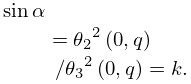… ►Tables of Neville’s theta functions ${\theta }_s(x,q)$, ${\theta }_c(x,q)$, ${\theta }_d(x,q)$, ${\theta }_n(x,q)$ (see §20.1) and their logarithmic $x$-derivatives are given in Abramowitz and Stegun (1964, pp. 582–585) to 9D for $\epsilon ,\alpha =0(5^{\circ }){90}^{\circ }$, where (in radian measure) $\epsilon =x/{\theta }_3^2(0,q)=\pi x/(2K\left(k\right))$, and $\alpha$ is defined by (20.15.1). …

34: 22.15 Inverse Functions

… ►

22.15.3 $$\mathrm{dn}(\zeta ,k)=x,$$ $k^{\prime }\le x\le 1$,

ⓘ

Symbols:

$\mathrm{dn}(z,k)$: Jacobian elliptic function, $x$: real, $k$: modulus, $k^{\prime }$: complementary modulus and $\zeta$: solution

Referenced by:

§22.15(i)

Permalink:

http://dlmf.nist.gov/22.15.E3

Encodings:

pMML, png, TeX

See also:

Annotations for §22.15(i), §22.15 and Ch.22

… ►

22.15.13 $$\mathrm{arccn}(x,k)={\int }_x^1\frac{dt}{\sqrt{(1-t^2)(k_{}^{\prime }{}_{}{}^2+k^2{t}^2)}},$$ $-1\le x\le 1$,

ⓘ

Symbols:

$dx$: differential of $x$ , $\int$: integral, $\mathrm{arccn}(x,k)$: inverse Jacobian elliptic function, $x$: real, $k$: modulus and $k^{\prime }$: complementary modulus

A&S Ref:

17.4.52

Referenced by:

§22.15(i)

Permalink:

http://dlmf.nist.gov/22.15.E13

Encodings:

pMML, png, TeX

See also:

Annotations for §22.15(ii), §22.15 and Ch.22

►

22.15.14 $$\mathrm{arcdn}(x,k)={\int }_x^1\frac{dt}{\sqrt{(1-t^2)(t^2-k_{}^{\prime }{}_{}{}^2)}},$$ $k^{\prime }\le x\le 1$ .

ⓘ

Symbols:

$dx$: differential of $x$ , $\int$: integral, $\mathrm{arcdn}(x,k)$: inverse Jacobian elliptic function, $x$: real, $k$: modulus and $k^{\prime }$: complementary modulus

A&S Ref:

17.4.44

Referenced by:

§22.15(ii)

Permalink:

http://dlmf.nist.gov/22.15.E14

Encodings:

pMML, png, TeX

See also:

Annotations for §22.15(ii), §22.15 and Ch.22

… ►

22.15.16 $$\mathrm{arcsd}(x,k)={\int }_0^x\frac{dt}{\sqrt{(1-k_{}^{\prime }{}_{}{}^2{t}^2)(1+k^2{t}^2)}},$$ $-1/k^{\prime }\le x\le 1/k^{\prime }$,

ⓘ

Symbols:

$dx$: differential of $x$ , $\int$: integral, $\mathrm{arcsd}(x,k)$: inverse Jacobian elliptic function, $x$: real, $k$: modulus and $k^{\prime }$: complementary modulus

A&S Ref:

17.4.51

Permalink:

http://dlmf.nist.gov/22.15.E16

Encodings:

pMML, png, TeX

See also:

Annotations for §22.15(ii), §22.15 and Ch.22

►

22.15.17 $$\mathrm{arcnd}(x,k)={\int }_1^x\frac{dt}{\sqrt{(t^2-1)(1-k_{}^{\prime }{}_{}{}^2{t}^2)}},$$ $1\le x\le 1/k^{\prime }$,

ⓘ

Symbols:

$dx$: differential of $x$ , $\int$: integral, $\mathrm{arcnd}(x,k)$: inverse Jacobian elliptic function, $x$: real, $k$: modulus and $k^{\prime }$: complementary modulus

A&S Ref:

17.4.43

Permalink:

http://dlmf.nist.gov/22.15.E17

Encodings:

pMML, png, TeX

See also:

Annotations for §22.15(ii), §22.15 and Ch.22

…

35: 33.10 Limiting Forms for Large $\rho$ or Large $\left|\eta \right|$

… ►

$$G_0(\eta ,\rho )\sim 2{\mathrm{e}}^{\pi \eta }{\left(\rho /\pi \right)}^{1/2}{K}_1\left({(8\eta \rho )}^{1/2}\right),$$

… ►

$$G_0^{\prime }(\eta ,\rho )\sim -2{\mathrm{e}}^{\pi \eta }{\left(2\eta /\pi \right)}^{1/2}{K}_0\left({(8\eta \rho )}^{1/2}\right).$$

… ►

$$F_0(\eta ,\rho )={(\pi \rho )}^{1/2}{J}_1\left({(-8\eta \rho )}^{1/2}\right)+o\left({\left|\eta \right|}^{-1/4}\right),$$

►

$$G_0(\eta ,\rho )=-{(\pi \rho )}^{1/2}{Y}_1\left({(-8\eta \rho )}^{1/2}\right)+o\left({\left|\eta \right|}^{-1/4}\right).$$

►

$$F_0^{\prime }(\eta ,\rho )={(-2\pi \eta )}^{1/2}{J}_0\left({(-8\eta \rho )}^{1/2}\right)+o\left({\left|\eta \right|}^{1/4}\right),$$

…

36: 14.22 Graphics

… ►

►

►

Figure 14.22.1: $P_{1/2}^0\left(x+\mathrm{i}y\right)$, $-5\le x\le 5$, $-5\le y\le 5$. … Magnify 3D Help

►

►

►

Figure 14.22.2: $P_{1/2}^{-1/2}\left(x+\mathrm{i}y\right)$, $-5\le x\le 5$, $-5\le y\le 5$. … Magnify 3D Help

►

►

►

Figure 14.22.3: $P_{1/2}^{-1}\left(x+\mathrm{i}y\right)$, $-5\le x\le 5$, $-5\le y\le 5$. … Magnify 3D Help

…

37: 22.6 Elementary Identities

… ►

22.6.3 $$k_{}^{\prime }{}_{}{}^2{\mathrm{sc}}^2(z,k)+1={\mathrm{dc}}^2(z,k)=k_{}^{\prime }{}_{}{}^2{\mathrm{nc}}^2(z,k)+k^2,$$

ⓘ

Symbols:

$\mathrm{dc}(z,k)$: Jacobian elliptic function, $\mathrm{nc}(z,k)$: Jacobian elliptic function, $\mathrm{sc}(z,k)$: Jacobian elliptic function, $z$: complex, $k$: modulus and $k^{\prime }$: complementary modulus

A&S Ref:

16.9.3

Permalink:

http://dlmf.nist.gov/22.6.E3

Encodings:

pMML, png, TeX

See also:

Annotations for §22.6(i), §22.6 and Ch.22

►

22.6.4 $$-k^{2}k_{}^{\prime }{}_{}{}^2{\mathrm{sd}}^2(z,k)=k^2({\mathrm{cd}}^2(z,k)-1)=k_{}^{\prime }{}_{}{}^2(1-{\mathrm{nd}}^2(z,k)).$$

ⓘ

Symbols:

$\mathrm{cd}(z,k)$: Jacobian elliptic function, $\mathrm{nd}(z,k)$: Jacobian elliptic function, $\mathrm{sd}(z,k)$: Jacobian elliptic function, $z$: complex, $k$: modulus and $k^{\prime }$: complementary modulus

A&S Ref:

16.9.2

Permalink:

http://dlmf.nist.gov/22.6.E4

Encodings:

pMML, png, TeX

See also:

Annotations for §22.6(i), §22.6 and Ch.22

… ►

22.6.8 $$\mathrm{cd}(2z,k)=\frac{{\mathrm{cd}}^2(z,k)-k_{}^{\prime }{}_{}{}^2{\mathrm{sd}}^2(z,k){\mathrm{nd}}^2(z,k)}{1+k^{2}k_{}^{\prime }{}_{}{}^2{\mathrm{sd}}^4(z,k)},$$

ⓘ

Symbols:

$\mathrm{cd}(z,k)$: Jacobian elliptic function, $\mathrm{nd}(z,k)$: Jacobian elliptic function, $\mathrm{sd}(z,k)$: Jacobian elliptic function, $z$: complex, $k$: modulus and $k^{\prime }$: complementary modulus

Permalink:

http://dlmf.nist.gov/22.6.E8

Encodings:

pMML, png, TeX

See also:

Annotations for §22.6(ii), §22.6 and Ch.22

►

22.6.9 $$\mathrm{sd}(2z,k)=\frac{2\mathrm{sd}(z,k)\mathrm{cd}(z,k)\mathrm{nd}(z,k)}{1+k^{2}k_{}^{\prime }{}_{}{}^2{\mathrm{sd}}^4(z,k)},$$

ⓘ

Symbols:

$\mathrm{cd}(z,k)$: Jacobian elliptic function, $\mathrm{nd}(z,k)$: Jacobian elliptic function, $\mathrm{sd}(z,k)$: Jacobian elliptic function, $z$: complex, $k$: modulus and $k^{\prime }$: complementary modulus

Permalink:

http://dlmf.nist.gov/22.6.E9

Encodings:

pMML, png, TeX

See also:

Annotations for §22.6(ii), §22.6 and Ch.22

… ►

§22.6(v) Change of Modulus

…

38: 19.4 Derivatives and Differential Equations

… ►

19.4.3 $$\frac{d^{2}E\left(k\right)}{{dk}^2}=-\frac{1}{k}\frac{dK\left(k\right)}{dk}=\frac{k_{}^{\prime }{}_{}{}^{2}K\left(k\right)-E\left(k\right)}{k^{2}k_{}^{\prime }{}_{}{}^2},$$

ⓘ

Symbols:

$K\left(k\right)$: Legendre’s complete elliptic integral of the first kind, $E\left(k\right)$: Legendre’s complete elliptic integral of the second kind, $\frac{df}{dx}$: derivative of $f$ with respect to $x$ , $k$: real or complex modulus and $k^{\prime }$: complementary modulus

Permalink:

http://dlmf.nist.gov/19.4.E3

Encodings:

pMML, png, TeX

See also:

Annotations for §19.4(i), §19.4 and Ch.19

… ►Let $D_k=\partial /\partial k$. … ►

19.4.8 $$(kk_{}^{\prime }{}_{}{}^2{D}_k^2+(1-3k^2)D_k-k)F(\varphi ,k)=\frac{-k\sin \varphi \cos \varphi }{{(1-k^2{\sin }^2\varphi )}^{3/2}},$$

ⓘ

Symbols:

$\cos z$: cosine function, $F(\varphi ,k)$: Legendre’s incomplete elliptic integral of the first kind, $\sin z$: sine function, $\varphi$: real or complex argument, $k$: real or complex modulus, $k^{\prime }$: complementary modulus and $D_k$: differential operator

Referenced by:

§19.4(ii)

Permalink:

http://dlmf.nist.gov/19.4.E8

Encodings:

pMML, png, TeX

See also:

Annotations for §19.4(ii), §19.4 and Ch.19

►

19.4.9 $$(kk_{}^{\prime }{}_{}{}^2{D}_k^2+k_{}^{\prime }{}_{}{}^2{D}_k+k)E(\varphi ,k)=\frac{k\sin \varphi \cos \varphi }{\sqrt{1-k^2{\sin }^2\varphi }}.$$

ⓘ

Symbols:

$\cos z$: cosine function, $E(\varphi ,k)$: Legendre’s incomplete elliptic integral of the second kind, $\sin z$: sine function, $\varphi$: real or complex argument, $k$: real or complex modulus, $k^{\prime }$: complementary modulus and $D_k$: differential operator

Permalink:

http://dlmf.nist.gov/19.4.E9

Encodings:

pMML, png, TeX

See also:

Annotations for §19.4(ii), §19.4 and Ch.19

►If $\varphi =\pi /2$, then these two equations become hypergeometric differential equations (15.10.1) for $K\left(k\right)$ and $E\left(k\right)$. …

39: 19.3 Graphics

… ►

►►

Figure 19.3.2: $R_C(x,1)$ and the Cauchy principal value of $R_C(x,-1)$ for $0\le x\le 5$. Both functions are asymptotic to $\ln \left(4x\right)/\sqrt{4x}$ as $x\to \mathrm{\infty }$; see (19.2.19) and (19.2.20). … Magnify

►

►

►

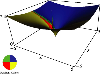
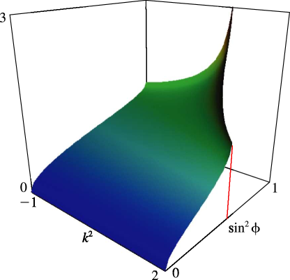
Figure 19.3.3: $F(\varphi ,k)$ as a function of $k^2$ and ${\sin }^2\varphi$ for $-1\le k^2\le 2$, $0\le {\sin }^2\varphi \le 1$. …If ${\sin }^2\varphi =1/k^2$ (), then it has the value $K\left(1/k\right)/k$: put $c=k^2$ in (19.25.5) and use (19.25.1). Magnify 3D Help

►

►

►

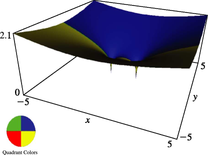
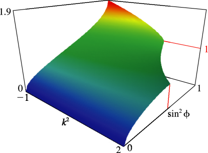
Figure 19.3.4: $E(\varphi ,k)$ as a function of $k^2$ and ${\sin }^2\varphi$ for $-1\le k^2\le 2$, $0\le {\sin }^2\varphi \le 1$. …If ${\sin }^2\varphi =1/k^2$ (), then it has the value $kE\left(1/k\right)+(k_{}^{\prime }{}_{}{}^2/k)K\left(1/k\right)$, with limit 1 as $k^2\to 1+$: put $c=k^2$ in (19.25.7) and use (19.25.1). Magnify 3D Help

… ►

►

►

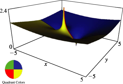
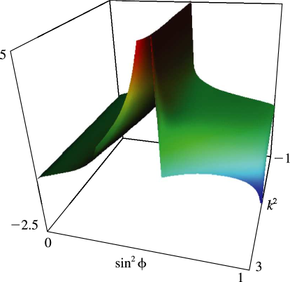
Figure 19.3.6: $\mathrm{\Pi }(\varphi ,2,k)$ as a function of $k^2$ and ${\sin }^2\varphi$ for $-1\le k^2\le 3$, . …If ${\sin }^2\varphi =1/k^2$ (), then by (19.7.4) it reduces to $\mathrm{\Pi }(2/k^2,1/k)/k$, $k^2\ne 2$, with Cauchy principal value $(K\left(1/k\right)-\mathrm{\Pi }(\frac{1}{2},1/k))/k$, , by (19.6.5). … Magnify 3D Help

… ►

►

►

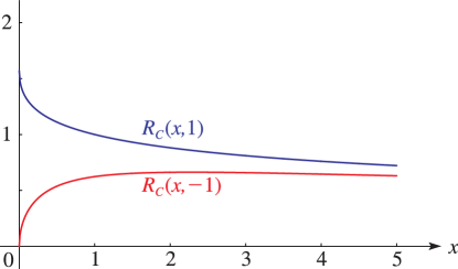
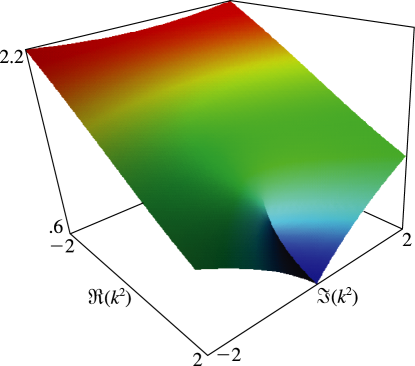
Figure 19.3.11: $\mathrm{\Re }\left(E\left(k\right)\right)$ as a function of complex $k^2$ for $-2\le \mathrm{\Re }\left(k^2\right)\le 2$, $-2\le \mathrm{\Im }\left(k^2\right)\le 2$. …On the branch cut ($k^2>1$) it has the value $kE\left(1/k\right)+(k_{}^{\prime }{}_{}{}^2/k)K\left(1/k\right)$, with limit 1 as $k^2\to 1+$. Magnify 3D Help

…

40: 21.1 Special Notation

… ► ►►►

$g,h$	positive integers.
…
$S_1/S_2$	set of all elements of $S_1$, modulo elements of $S_2$. Thus two elements of $S_1/S_2$ are equivalent if they are both in $S_1$ and their difference is in $S_2$. (For an example see §20.12(ii).)
…

… ►The function $\mathrm{\Theta }(\mathit{\varphi }|𝐁)=\theta \left(\mathit{\varphi }/(2\pi \mathrm{i})\right|𝐁/(2\pi \mathrm{i}))$ is also commonly used; see, for example, Belokolos et al. (1994, §2.5), Dubrovin (1981), and Fay (1973, Chapter 1).