interrelation between bases

SearchAdvancedHelp

(0.002 seconds)

11—20 of 428 matching pages

11: 8.21 Generalized Sine and Cosine Integrals

… ►

8.21.1 $$\mathrm{ci}(a,z)\pm \mathrm{i}\mathrm{si}(a,z)={\mathrm{e}}^{\pm \frac{1}{2}\pi \mathrm{i}a}\mathrm{\Gamma }(a,z{\mathrm{e}}^{\mp \frac{1}{2}\pi \mathrm{i}}),$$

ⓘ

Defines:

$\mathrm{ci}(a,z)$: generalized cosine integral and $\mathrm{si}(a,z)$: generalized sine integral

Symbols:

$\pi$: the ratio of the circumference of a circle to its diameter, $\mathrm{e}$: base of natural logarithm, $\mathrm{i}$: imaginary unit, $\mathrm{\Gamma }(a,z)$: incomplete gamma function, $z$: complex variable and $a$: parameter

Referenced by:

§8.21(ii)

Permalink:

http://dlmf.nist.gov/8.21.E1

Encodings:

pMML, png, TeX

See also:

Annotations for §8.21(i), §8.21 and Ch.8

… ►

8.21.3 $${\int }_0^{\mathrm{\infty }}{t}^{a-1}{\mathrm{e}}^{\pm \mathrm{i}t}dt={\mathrm{e}}^{\pm \frac{1}{2}\pi \mathrm{i}a}\mathrm{\Gamma }\left(a\right),$$ ,

ⓘ

Symbols:

$\mathrm{\Gamma }\left(z\right)$: gamma function, $\pi$: the ratio of the circumference of a circle to its diameter, $dx$: differential of $x$ , $\mathrm{e}$: base of natural logarithm, $\mathrm{i}$: imaginary unit, $\int$: integral, $\mathrm{\Re }$: real part and $a$: parameter

Referenced by:

§8.21(iv)

Permalink:

http://dlmf.nist.gov/8.21.E3

Encodings:

pMML, png, TeX

See also:

Annotations for §8.21(ii), §8.21 and Ch.8

… ►

§8.21(iv) Interrelations

… ►

8.21.24 $$f(a,z)=\frac{z^a}{2}{\int }_0^{\mathrm{\infty }}\left({(1+\mathrm{i}t)}^{a-1}+{(1-\mathrm{i}t)}^{a-1}\right){\mathrm{e}}^{-zt}dt,$$

ⓘ

Symbols:

$dx$: differential of $x$ , $\mathrm{e}$: base of natural logarithm, $\mathrm{i}$: imaginary unit, $\int$: integral, $z$: complex variable, $a$: parameter and $f(a,z)$: auxiliary function

Referenced by:

§8.21(vii), §8.21(viii)

Permalink:

http://dlmf.nist.gov/8.21.E24

Encodings:

pMML, png, TeX

See also:

Annotations for §8.21(vii), §8.21 and Ch.8

►

8.21.25 $$g(a,z)=\frac{z^a}{2\mathrm{i}}{\int }_0^{\mathrm{\infty }}\left({(1-\mathrm{i}t)}^{a-1}-{(1+\mathrm{i}t)}^{a-1}\right){\mathrm{e}}^{-zt}dt.$$

ⓘ

Symbols:

$dx$: differential of $x$ , $\mathrm{e}$: base of natural logarithm, $\mathrm{i}$: imaginary unit, $\int$: integral, $z$: complex variable, $a$: parameter and $g(a,z)$: auxiliary function

Referenced by:

§8.21(vii), §8.21(viii)

Permalink:

http://dlmf.nist.gov/8.21.E25

Encodings:

pMML, png, TeX

See also:

Annotations for §8.21(vii), §8.21 and Ch.8

…

12: 18.11 Relations to Other Functions

… ►

Ultraspherical

… ►

18.11.2 $$L_n^{(\alpha )}\left(x\right)=\frac{{\left(\alpha +1\right)}_n}{n!}M(-n,\alpha +1,x)=\frac{{(-1)}^n}{n!}U(-n,\alpha +1,x)=\frac{{\left(\alpha +1\right)}_n}{n!}{x}^{-\frac{1}{2}(\alpha +1)}{\mathrm{e}}^{\frac{1}{2}x}{M}_{n+\frac{1}{2}(\alpha +1),\frac{1}{2}\alpha }\left(x\right)=\frac{{(-1)}^n}{n!}{x}^{-\frac{1}{2}(\alpha +1)}{\mathrm{e}}^{\frac{1}{2}x}{W}_{n+\frac{1}{2}(\alpha +1),\frac{1}{2}\alpha }\left(x\right).$$

ⓘ

Symbols:

$M(a,b,z)$: $={}_1{}^{}F_1^{}(a;b;z)$ Kummer confluent hypergeometric function, $U(a,b,z)$: Kummer confluent hypergeometric function, $L_n^{(\alpha )}\left(x\right)$: Laguerre (or generalized Laguerre) polynomial, ${\left(a\right)}_n$: Pochhammer’s symbol (or shifted factorial), $M_{\kappa ,\mu }\left(z\right)$: Whittaker confluent hypergeometric function, $W_{\kappa ,\mu }\left(z\right)$: Whittaker confluent hypergeometric function, $\mathrm{e}$: base of natural logarithm, $!$: factorial (as in $n!$), $n$: nonnegative integer and $x$: real variable

Referenced by:

§13.6(v), §18.11(i)

Permalink:

http://dlmf.nist.gov/18.11.E2

Encodings:

pMML, png, TeX

See also:

Annotations for §18.11(i), §18.11(i), §18.11 and Ch.18

… ►

18.11.3 $$H_n\left(x\right)=2^{n}U(-\frac{1}{2}n,\frac{1}{2},x^2)=2^{n}xU(-\frac{1}{2}n+\frac{1}{2},\frac{3}{2},x^2)=2^{\frac{1}{2}n}{\mathrm{e}}^{\frac{1}{2}{x}^2}U(-n-\frac{1}{2},2^{\frac{1}{2}}x),$$

ⓘ

Symbols:

$H_n\left(x\right)$: Hermite polynomial, $U(a,b,z)$: Kummer confluent hypergeometric function, $\mathrm{e}$: base of natural logarithm, $U(a,z)$: parabolic cylinder function, $n$: nonnegative integer and $x$: real variable

A&S Ref:

22.5.55, 22.5.58 ((factor $x$ missing on RHS of 22.5.55))

Referenced by:

§18.11(i), §18.15(v)

Permalink:

http://dlmf.nist.gov/18.11.E3

Encodings:

pMML, png, TeX

See also:

Annotations for §18.11(i), §18.11(i), §18.11 and Ch.18

►

18.11.4 $${\mathrm{𝐻𝑒}}_n\left(x\right)=2^{\frac{1}{2}n}U(-\frac{1}{2}n,\frac{1}{2},\frac{1}{2}{x}^2)=2^{\frac{1}{2}(n-1)}xU(-\frac{1}{2}n+\frac{1}{2},\frac{3}{2},\frac{1}{2}{x}^2)={\mathrm{e}}^{\frac{1}{4}{x}^2}U(-n-\frac{1}{2},x).$$

ⓘ

Symbols:

${\mathrm{𝐻𝑒}}_n\left(x\right)$: Hermite polynomial, $U(a,b,z)$: Kummer confluent hypergeometric function, $\mathrm{e}$: base of natural logarithm, $U(a,z)$: parabolic cylinder function, $n$: nonnegative integer and $x$: real variable

A&S Ref:

22.5.59

Permalink:

http://dlmf.nist.gov/18.11.E4

Encodings:

pMML, png, TeX

See also:

Annotations for §18.11(i), §18.11(i), §18.11 and Ch.18

…

13: 32.7 Bäcklund Transformations

§32.7 Bäcklund Transformations

… ►

§32.7(vi) Relationship Between the Third and Fifth Painlevé Equations

… ► …

14: 4.23 Inverse Trigonometric Functions

… ►

§4.23(vii) Special Values and Interrelations

… ►For interrelations see Table 4.16.3. … ►

4.23.40 $$\mathrm{gd}\left(x\right)=2\arctan \left({\mathrm{e}}^x\right)-\frac{1}{2}\pi =\arcsin \left(\tanh x\right)=\mathrm{arccsc}\left(\coth x\right)=\arccos \left(\mathrm{sech}x\right)=\mathrm{arcsec}\left(\cosh x\right)=\arctan \left(\sinh x\right)=\mathrm{arccot}\left(\mathrm{csch}x\right).$$

ⓘ

Symbols:

$\mathrm{gd}x$: Gudermannian function, $\pi$: the ratio of the circumference of a circle to its diameter, $\mathrm{e}$: base of natural logarithm, $\mathrm{csch}z$: hyperbolic cosecant function, $\cosh z$: hyperbolic cosine function, $\coth z$: hyperbolic cotangent function, $\mathrm{sech}z$: hyperbolic secant function, $\sinh z$: hyperbolic sine function, $\tanh z$: hyperbolic tangent function, $\mathrm{arccsc}z$: arccosecant function, $\arccos z$: arccosine function, $\mathrm{arccot}z$: arccotangent function, $\mathrm{arcsec}z$: arcsecant function, $\arcsin z$: arcsine function, $\arctan z$: arctangent function and $x$: real variable

Referenced by:

§4.23(viii), §4.40(ii)

Permalink:

http://dlmf.nist.gov/4.23.E40

Encodings:

pMML, png, TeX

See also:

Annotations for §4.23(viii), §4.23 and Ch.4

…

15: 4.30 Elementary Properties

… ►

Table 4.30.1: Hyperbolic functions: interrelations. …

► ►►

	$\sinh \theta =a$	$\cosh \theta =a$	$\tanh \theta =a$	$\mathrm{csch}\theta =a$	$\mathrm{sech}\theta =a$	$\coth \theta =a$
…

►

16: 11.10 Anger–Weber Functions

… ►

11.10.4 $${𝐀}_{\nu }\left(z\right)=\frac{1}{\pi }{\int }_0^{\mathrm{\infty }}{\mathrm{e}}^{-\nu t-z\sinh t}dt,$$ $\mathrm{\Re }z>0$.

ⓘ

Defines:

${𝐀}_{\nu }\left(z\right)$: Anger–Weber function

Symbols:

$\pi$: the ratio of the circumference of a circle to its diameter, $dx$: differential of $x$ , $\mathrm{e}$: base of natural logarithm, $\sinh z$: hyperbolic sine function, $\int$: integral, $\mathrm{\Re }$: real part, $z$: complex variable and $\nu$: real or complex order

Referenced by:

§11.10(i), (11.11.10), (11.11.11), §11.11(iii)

Permalink:

http://dlmf.nist.gov/11.10.E4

Encodings:

pMML, png, TeX

See also:

Annotations for §11.10(i), §11.10 and Ch.11

… ►

§11.10(v) Interrelations

…

17: 35.9 Applications

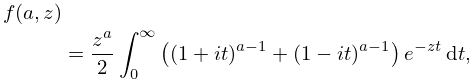
… ►In multivariate statistical analysis based on the multivariate normal distribution, the probability density functions of many random matrices are expressible in terms of generalized hypergeometric functions of matrix argument ${}_p{}^{}F_q^{}$, with $p\le 2$ and $q\le 1$. … ►For applications of the integral representation (35.5.3) see McFarland and Richards (2001, 2002) (statistical estimation of misclassification probabilities for discriminating between multivariate normal populations). …

18: 4.3 Graphics

… ►

►►

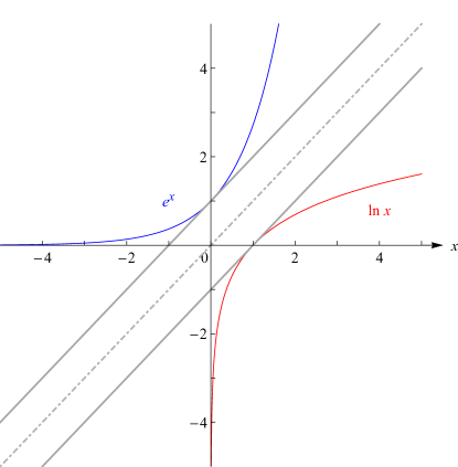
Figure 4.3.1: $\ln x$ and ${\mathrm{e}}^x$. Parallel tangent lines at $(1,0)$ and $(0,1)$ make evident the mirror symmetry across the line $y=x$, demonstrating the inverse relationship between the two functions. Magnify

…

19: 28.27 Addition Theorems

… ►Addition theorems provide important connections between Mathieu functions with different parameters and in different coordinate systems. …

20: 7.20 Mathematical Applications

… ►Then the arc length between the origin and $P(t)$ equals $t$, and is directly proportional to the curvature at $P(t)$, which equals $\pi t$. Furthermore, because $dy/dx=\tan \left(\frac{1}{2}\pi t^2\right)$, the angle between the $x$-axis and the tangent to the spiral at $P(t)$ is given by $\frac{1}{2}\pi t^2$. … ►

7.20.1 $$\frac{1}{\sigma \sqrt{2\pi }}{\int }_{-\mathrm{\infty }}^x{\mathrm{e}}^{-{(t-m)}^2/(2{\sigma }^2)}dt=\frac{1}{2}\mathrm{erfc}\left(\frac{m-x}{\sigma \sqrt{2}}\right)=Q\left(\frac{m-x}{\sigma }\right)=P\left(\frac{x-m}{\sigma }\right).$$

ⓘ

Symbols:

$\pi$: the ratio of the circumference of a circle to its diameter, $\mathrm{erfc}z$: complementary error function, $dx$: differential of $x$ , $\mathrm{e}$: base of natural logarithm, $\int$: integral, $x$: real variable, $m$: mean and $\sigma$: standard deviation

A&S Ref:

7.1.22 (slightly modified)

Permalink:

http://dlmf.nist.gov/7.20.E1

Encodings:

pMML, png, TeX

See also:

Annotations for §7.20(iii), §7.20 and Ch.7

…