integral equations

SearchAdvancedHelp

(0.010 seconds)

31—40 of 215 matching pages

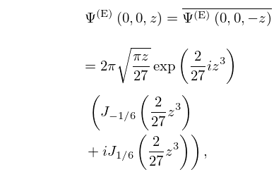
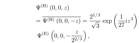
31: 9.13 Generalized Airy Functions

… ►Reid (1972) and Drazin and Reid (1981, Appendix) introduce the following contour integrals in constructing approximate solutions to the Orr–Sommerfeld equation for fluid flow: … ►Each of the functions $A_k(z,p)$ and $B_k(z,p)$ satisfies the differential equation …and the difference equation …

32: Errata

… ►

18.28.2 $${\int }_{-1}^1{p}_n(x)p_m(x)w(x)dx=h_n{\delta }_{n,m},$$ $|a|,|b|,|c|,|d|\le 1$, $ab,ac,ad,bc,bd,cd\ne 1$

The constraint of this equation was updated to include $ab,ac,ad,bc,bd,cd\ne 1$.

… ►

The following additions were made in Chapter 1:

• New subsections, 1.2(v) Matrices, Vectors, Scalar Products, and Norms and 1.2(vi) Square Matrices, with Equations (1.2.27)–(1.2.77).

• The title of this section was changed from “Determinants” to “Determinants, Linear Operators, and Spectral Expansions”. An extra paragraph just below (1.3.7). New subsection, 1.3(iv) Matrices as Linear Operators, with Equations (1.3.20), (1.3.21).

• In 1.4(v), three new paragraphs on Stieltjes integrals/measure, with Equations (1.4.23_1)–(1.4.23_3).

• In Subsection 1.8(i), the title of the paragraph “Bessel’s Inequality” was changed to “Parseval’s Formula”. We give the relation between the real and the complex coefficients, and include more general versions of Parseval’s Formula, Equations (1.8.6_1), (1.8.6_2). The title of Subsection 1.8(iv) was changed from “Transformations” to “Poisson’s Summation Formula”, and we added an extra remark just below (1.8.14).

• New subsection, 1.10(xi) Generating Functions, with Equations (1.10.26)–(1.10.29).

• New subsection, 1.13(viii) Eigenvalues and Eigenfunctions: Sturm-Liouville and Liouville forms, with Equations (1.13.26)–(1.13.31).

• Another form of Parseval’s formula, (1.14.7_5).

• We include several extra remarks and Equations (1.16.3_5), (1.16.9_5). New subsection, 1.16(ix) References for Section 1.16.

• Two extra paragraphs in Subsection 1.17(ii) Integral Representations, with Equations (1.17.12_1), (1.17.12_2); Subsection 1.17(iv) Mathematical Definitions is almost completely rewritten.

• An entire new section, 1.18 Linear Second Order Differential Operators and Eigenfunction Expansions, including new subsections, 1.18(i)–1.18(x), and several equations, (1.18.1)–(1.18.71).

… ►

Section: 15.9(v) Complete Elliptic Integrals. Equations: (11.11.9_5), (11.11.13_5), Intermediate equality in (15.4.27) which relates to $F(a,a;a+1;\frac{1}{2})$, (15.4.34), (19.5.4_1), (19.5.4_2) and (19.5.4_3).

… ►

33.14.15 $${\int }_0^{\mathrm{\infty }}{\varphi }_{m,\mathrm{\ell }}(r){\varphi }_{n,\mathrm{\ell }}(r)dr={\delta }_{m,n}$$

The definite integral, originally written as ${\int }_0^{\mathrm{\infty }}{\varphi }_{n,\mathrm{\ell }}^2(r)dr=1$, was clarified and rewritten as an orthogonality relation. This follows from (33.14.14) by combining it with Dunkl (2003, Theorem 2.2).

… ►

A sentence and unnumbered equation

$$R_C(\gamma -\delta ,\gamma )=\frac{-1}{\sqrt{\delta }}\arctan \left(\frac{\sqrt{\delta }\sin \theta \sin \varphi \sin \psi }{{\alpha }^2-1-{\alpha }^2\cos \theta \cos \varphi \cos \psi }\right),$$

were added which indicate that care must be taken with the multivalued functions in (19.11.5). See (Cayley, 1961, pp. 103-106).

Suggested by Albert Groenenboom.

…

33: 28.6 Expansions for Small $q$

… ►where $k$ is the unique root of the equation $2E\left(k\right)=K\left(k\right)$ in the interval $(0,1)$, and $k^{\prime }=\sqrt{1-k^2}$. …

34: 36.2 Catastrophes and Canonical Integrals

… ►

36.2.28 $${\mathrm{\Psi }}^{(\mathrm{E})}\left(0,0,z\right)=\overline{{\mathrm{\Psi }}^{(\mathrm{E})}\left(0,0,-z\right)}=2\pi \sqrt{\frac{\pi z}{27}}\exp \left(\frac{2}{27}\mathrm{i}{z}^3\right)\left(J_{-1/6}\left(\frac{2}{27}{z}^3\right)+\mathrm{i}{J}_{1/6}\left(\frac{2}{27}{z}^3\right)\right),$$ $z\ge 0$,

ⓘ

Symbols:

$J_{\nu }\left(z\right)$: Bessel function of the first kind, $\pi$: the ratio of the circumference of a circle to its diameter, $\overline{z}$: complex conjugate, ${\mathrm{\Psi }}^{(\mathrm{E})}\left(𝐱\right)$: elliptic umbilic canonical integral function, $\exp z$: exponential function, $\mathrm{i}$: imaginary unit and $z$: real parameter

Referenced by:

Erratum (V1.0.5) for Chapters 8, 20, 36

Permalink:

http://dlmf.nist.gov/36.2.E28

Encodings:

pMML, png, TeX

Addition (effective with 1.0.5):

This equation has been added. For the proof see Berry and Howls (2010).

See also:

Annotations for §36.2(iv), §36.2 and Ch.36

►

36.2.29 $${\mathrm{\Psi }}^{(\mathrm{H})}\left(0,0,z\right)=\overline{{\mathrm{\Psi }}^{(\mathrm{H})}\left(0,0,-z\right)}=\frac{2^{1/3}}{\sqrt{3}}\exp \left(\frac{1}{27}\mathrm{i}{z}^3\right){\mathrm{\Psi }}^{(\mathrm{E})}\left(0,0,-\frac{z}{2^{2/3}}\right),$$ .

ⓘ

Symbols:

$\overline{z}$: complex conjugate, ${\mathrm{\Psi }}^{(\mathrm{E})}\left(𝐱\right)$: elliptic umbilic canonical integral function, $\exp z$: exponential function, ${\mathrm{\Psi }}^{(\mathrm{H})}\left(𝐱\right)$: hyperbolic umbilic canonical integral function, $\mathrm{i}$: imaginary unit and $z$: real parameter

Referenced by:

Erratum (V1.0.5) for Chapters 8, 20, 36

Permalink:

http://dlmf.nist.gov/36.2.E29

Encodings:

pMML, png, TeX

Addition (effective with 1.0.5):

This equation has been added. For the proof see Berry and Howls (2010).

See also:

Annotations for §36.2(iv), §36.2 and Ch.36

35: 25.14 Lerch’s Transcendent

… ►

25.14.5 $$\mathrm{\Phi }(z,s,a)=\frac{1}{\mathrm{\Gamma }\left(s\right)}{\int }_0^{\mathrm{\infty }}\frac{x^{s-1}{\mathrm{e}}^{-ax}}{1-z{\mathrm{e}}^{-x}}dx,$$ $\mathrm{\Re }s>1$, $\mathrm{\Re }a>0$ if $z=1$; $\mathrm{\Re }s>0$, $\mathrm{\Re }a>0$ if $z\in ℂ\setminus [1,\mathrm{\infty })$.

ⓘ

Symbols:

$\mathrm{\Gamma }\left(z\right)$: gamma function, $\mathrm{\Phi }(z,s,a)$: Lerch’s transcendent, $[a,b)$: half-closed interval, $ℂ$: complex plane, $dx$: differential of $x$ , $\in$: element of, $\mathrm{e}$: base of natural logarithm, $\int$: integral, $\mathrm{\Re }$: real part, $\setminus$: set subtraction, $x$: real variable, $a$: real or complex parameter, $s$: complex variable and $z$: complex variable

Keywords:

improper integral, integral representation

Source:

Erdélyi et al. (1953a, (1.11.3), p. 27)

Referenced by:

Erratum (V1.1.4) for Equation (25.14.5)

Permalink:

http://dlmf.nist.gov/25.14.E5

Encodings:

pMML, png, TeX

See also:

Annotations for §25.14(ii), §25.14 and Ch.25

►

25.14.6 $$\mathrm{\Phi }(z,s,a)=\frac{1}{2}{a}^{-s}+{\int }_0^{\mathrm{\infty }}\frac{z^x}{{(a+x)}^s}dx-2{\int }_0^{\mathrm{\infty }}\frac{\sin \left(x\ln z-s\arctan \left(x/a\right)\right)}{{(a^2+x^2)}^{s/2}({\mathrm{e}}^{2\pi x}-1)}dx,$$ $\mathrm{\Re }a>0$ if ; $\mathrm{\Re }s>1$, $\mathrm{\Re }a>0$ if $\left|z\right|=1$.

ⓘ

Symbols:

$\mathrm{\Phi }(z,s,a)$: Lerch’s transcendent, $\pi$: the ratio of the circumference of a circle to its diameter, $dx$: differential of $x$ , $\mathrm{e}$: base of natural logarithm, $\int$: integral, $\arctan z$: arctangent function, $\ln z$: principal branch of logarithm function, $\mathrm{\Re }$: real part, $\sin z$: sine function, $x$: real variable, $a$: real or complex parameter, $s$: complex variable and $z$: complex variable

Keywords:

improper integral, integral representation

Source:

Erdélyi et al. (1953a, (1.11.4), p. 28)

Notes:

For the case see Erdélyi et al. (1953a, (1.11.4), p. 28). In the case $\left|z\right|=1$ one checks that the first integral converges absolutely iff $\mathrm{\Re }s>1$.

Referenced by:

Erratum (V1.1.4) for Equation (25.14.6)

Permalink:

http://dlmf.nist.gov/25.14.E6

Encodings:

pMML, png, TeX

Clarification (effective with 1.1.4):

The constraint which originally read “$\mathrm{\Re }s>0$ if ; $\mathrm{\Re }s>1$ if $|z|=1,\mathrm{\Re }a>0$” has been improved to be “$\mathrm{\Re }a>0$ if ; $\mathrm{\Re }s>1$, $\mathrm{\Re }a>0$ if $\left|z\right|=1$”.

Suggested 2021-08-23 by Gergő Nemes

See also:

Annotations for §25.14(ii), §25.14 and Ch.25

…

36: 29.2 Differential Equations

… ►This equation has regular singularities at the points $2pK+(2q+1)\mathrm{i}{K}^{\prime }$, where $p,q\in \mathbb{Z}$, and $K$, $K^{\prime }$ are the complete elliptic integrals of the first kind with moduli $k$, $k^{\prime }(={(1-k^2)}^{1/2})$, respectively; see §19.2(ii). …

37: 22.19 Physical Applications

… ►

22.19.2 $$\sin \left(\frac{1}{2}\theta (t)\right)=\sin \left(\frac{1}{2}\alpha \right)\mathrm{sn}(t+K,\sin \left(\frac{1}{2}\alpha \right)),$$

ⓘ

Symbols:

$\mathrm{sn}(z,k)$: Jacobian elliptic function, $K\left(k\right)$: Legendre’s complete elliptic integral of the first kind, $\sin z$: sine function, $\theta (t)$: angular displacement and $\alpha$: initial displacement

Referenced by:

§22.19(i), §22.19(i), Erratum (V1.0.8) for Equation (22.19.2)

Permalink:

http://dlmf.nist.gov/22.19.E2

Encodings:

pMML, png, TeX

Errata (effective with 1.0.8):

Originally the first argument to the function $\mathrm{sn}$ was given incorrectly as $t$. The correct argument is $t+K$.

Reported 2014-03-05 by Svante Janson

See also:

Annotations for §22.19(i), §22.19 and Ch.22

… ►Hyperelliptic functions $u(z)$ are solutions of the equation $z={\int }_0^u{(f(x))}^{-1/2}dx$, where $f(x)$ is a polynomial of degree higher than 4. …

38: 32.4 Isomonodromy Problems

… ►Note that the right-hand side of the last equation is a first integral of the system (32.4.10)–(32.4.13). …

39: 22.16 Related Functions

… ►If $-K\le x\le K$, then the following four equations are equivalent: … ►

22.16.14 $$ℰ(x,k)={\int }_0^{\mathrm{sn}(x,k)}\sqrt{\frac{1-k^2{t}^2}{1-t^2}}dt;$$

ⓘ

Defines:

$ℰ(x,k)$: Jacobi’s epsilon function

Symbols:

$\mathrm{sn}(z,k)$: Jacobian elliptic function, $dx$: differential of $x$ , $\int$: integral, $x$: real and $k$: modulus

Referenced by:

§22.16(ii), Erratum (V1.0.1) for Equation (22.16.14)

Permalink:

http://dlmf.nist.gov/22.16.E14

Encodings:

pMML, png, TeX

Errata (effective with 1.0.1):

Originally appeared with the upper limit as $x$, rather than $\mathrm{sn}(x,k)$:

$$ℰ(x,k)={\int }_0^x\sqrt{\frac{1-k^2{t}^2}{1-t^2}}dt$$

Reported 2010-07-08 by Charles Karney

See also:

Annotations for §22.16(ii), §22.16(ii), §22.16 and Ch.22

… ►In Equations (22.16.21)–(22.16.23), … ►In Equations (22.16.24)–(22.16.26), . …

40: 6.2 Definitions and Interrelations

… ►

§6.2(i) Exponential and Logarithmic Integrals

… ► … ►The logarithmic integral is defined by … ►

§6.2(ii) Sine and Cosine Integrals

… ► …