integer degree and order
(0.003 seconds)
31—40 of 50 matching pages
31: Bibliography
…
►
Polygamma functions of negative order.
J. Comput. Appl. Math. 100 (2), pp. 191–199.
…
►
On the degrees of irreducible factors of higher order Bernoulli polynomials.
Acta Arith. 62 (4), pp. 329–342.
►
Congruences of -adic integer order Bernoulli numbers.
J. Number Theory 59 (2), pp. 374–388.
…
►
Algorithm 804: Subroutines for the computation of Mathieu functions of integer orders.
ACM Trans. Math. Software 26 (3), pp. 408–414.
…
►
Spherical Bessel functions and of integer order and real argument.
Comput. Phys. Comm. 14 (3-4), pp. 261–265.
…
32: 24.16 Generalizations
…
►
§24.16(i) Higher-Order Analogs
►Polynomials and Numbers of Integer Order
►For , Bernoulli and Euler polynomials of order are defined respectively by … ► is a polynomial in of degree . … ►In no particular order, other generalizations include: Bernoulli numbers and polynomials with arbitrary complex index (Butzer et al. (1992)); Euler numbers and polynomials with arbitrary complex index (Butzer et al. (1994)); q-analogs (Carlitz (1954a), Andrews and Foata (1980)); conjugate Bernoulli and Euler polynomials (Hauss (1997, 1998)); Bernoulli–Hurwitz numbers (Katz (1975)); poly-Bernoulli numbers (Kaneko (1997)); Universal Bernoulli numbers (Clarke (1989)); -adic integer order Bernoulli numbers (Adelberg (1996)); -adic -Bernoulli numbers (Kim and Kim (1999)); periodic Bernoulli numbers (Berndt (1975b)); cotangent numbers (Girstmair (1990b)); Bernoulli–Carlitz numbers (Goss (1978)); Bernoulli–Padé numbers (Dilcher (2002)); Bernoulli numbers belonging to periodic functions (Urbanowicz (1988)); cyclotomic Bernoulli numbers (Girstmair (1990a)); modified Bernoulli numbers (Zagier (1998)); higher-order Bernoulli and Euler polynomials with multiple parameters (Erdélyi et al. (1953a, §§1.13.1, 1.14.1)).33: 18.39 Applications in the Physical Sciences
…
►The nature of, and notations and common vocabulary for, the eigenvalues and eigenfunctions of self-adjoint second order differential operators is overviewed in §1.18.
…
►The fundamental quantum Schrödinger operator, also called the Hamiltonian, , is a second order differential operator of the form
…
►
is referred to as the ground state, all others, in order of increasing energy being excited states.
…
►Namely the th eigenfunction, listed in order of increasing eigenvalues, starting at , has precisely nodes, as real zeros of wave-functions away from boundaries are often referred to.
…
►Physical scientists use the of Bohr as, to th and st order, it describes the structure and organization of the Periodic Table of the Chemical Elements of which the Hydrogen atom is only the first.
…
34: 23.20 Mathematical Applications
…
►Let denote the set of points on that are of finite order (that is, those points for which there exists a positive integer
with ), and let be the sets of points with integer and rational coordinates, respectively.
…The resulting points are then tested for finite order as follows.
…If any of these quantities is zero, then the point has finite order.
If any of , , is not an integer, then the point has infinite order.
…
►The modular equation of degree
, prime, is an algebraic equation in and .
…
35: 13.2 Definitions and Basic Properties
…
►
Kummer’s Equation
… ►When , , is a polynomial in of degree not exceeding ; this is also true of provided that is not a nonpositive integer. … ►When , , is a polynomial in of degree : … ►When , … ►Also, when is not an integer …36: Frank W. J. Olver
…
►degrees in mathematics from the University of London in 1945, 1948, and 1961, respectively.
…
►Olver joined NIST in 1961 after having been recruited by Milton Abramowitz to be the author of the Chapter “Bessel Functions of Integer Order” in the Handbook of Mathematical Functions with Formulas, Graphs, and Mathematical Tables, a publication which went on to become the most widely distributed and most highly cited publication in NIST’s history.
…
37: Philip J. Davis
…
► 2018) received an undergraduate degree in mathematics from Harvard College in 1943.
…
►Olver had been recruited to write the Chapter “Bessel Functions of Integer Order” for A&S by Milton Abramowitz, who passed away suddenly in 1958.
…
38: Bibliography C
…
►
An algorithm for exponential integrals of real order.
Computing 45 (3), pp. 269–276.
…
►
The zeros of Hankel functions as functions of their order.
Numer. Math. 7 (3), pp. 238–250.
…
►
Derivatives with respect to the degree and order of associated Legendre functions for using modified Bessel functions.
Integral Transforms Spec. Funct. 21 (7-8), pp. 581–588.
…
►
Chazy’s second-degree Painlevé equations.
J. Phys. A 39 (39), pp. 11955–11971.
…
►
Zeros of the Hankel function of real order out of the principal Riemann sheet.
J. Comput. Appl. Math. 37 (1-3), pp. 89–99.
…
39: 18.15 Asymptotic Approximations
…
►
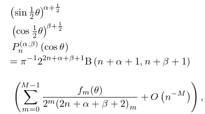
18.15.1
…
►
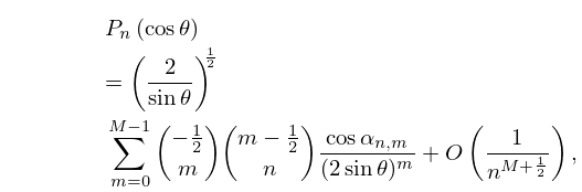
18.15.12
…
►
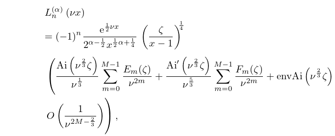
18.15.22
…
►
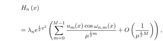
18.15.27
…
►The asymptotic behavior of the classical OP’s as with the degree and parameters fixed is evident from their explicit polynomial forms; see, for example, (18.2.7) and the last two columns of Table 18.3.1.
…
